24 Step-by-Step Tutorial

Authors: E.W. Hans and B. Alves de Brito Beirigo

This tutorial introduces Excel’s basic functionalities. You may be familiar with Excel to some extent. In that case, this manual probably still contains functionalities and tricks you did not know about. In any case, this manual is compiled from all functionalities that are deemed “useful” by students and staff from the BSc and MSc programs that use it. Your feedback and ideas for additions are therefore much appreciated!

24.1 Excel Installation

Microsoft Office 365 is available for UT students; you can access (via Cloud) and/or install:

Word
Excel
PowerPoint
Teams
Outlook
OneDrive

Learn more about obtaining MS Office 365 (Excel) at: https://www.utwente.nl/en/lisa/faq/office365-faq/.

24.2 Excel Interface and Settings

Fine Tuning the Interface and the Ribbon

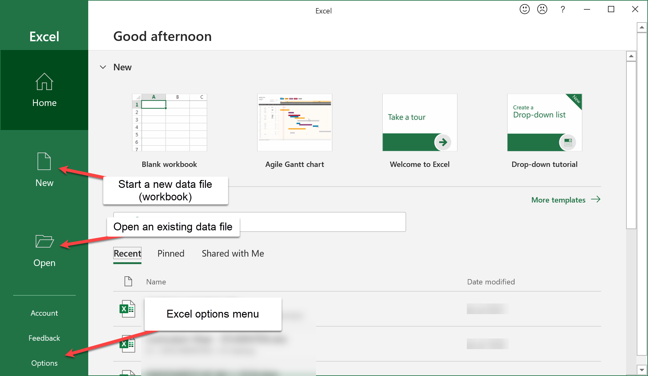
Start Excel via the Windows Start menu (press the windows key or click the windows menu button, and type “excel” to quickly find the Excel icon). After Excel has started, you see the following window, which allows you to create a new Excel data file (which is called a workbook), open an existing one, or open the Excel options menu (see below).

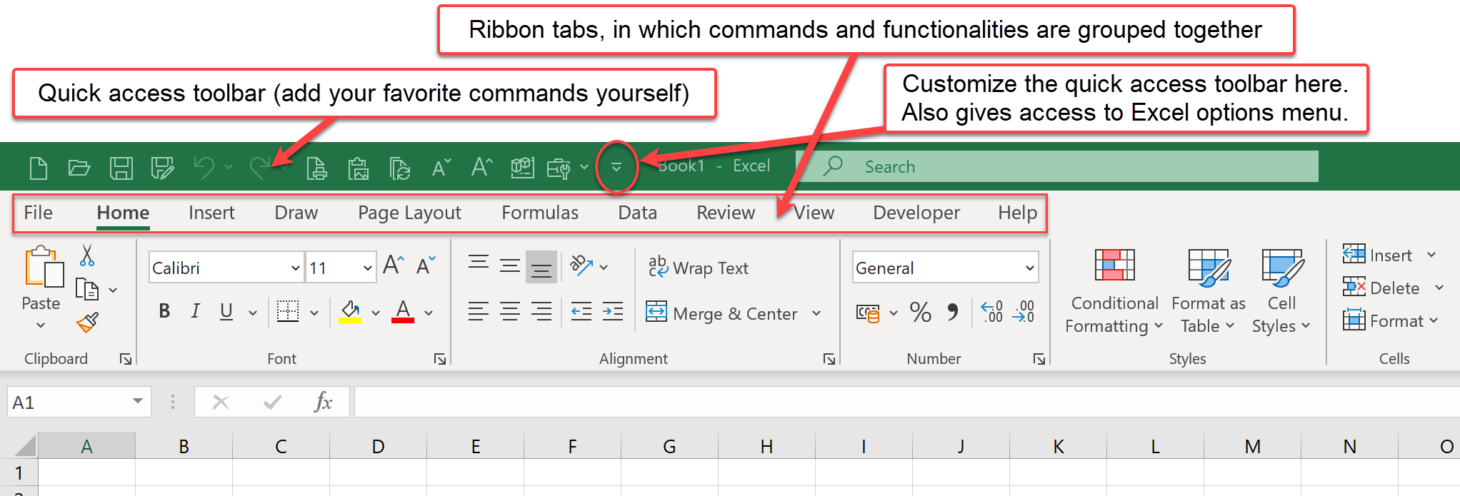
Once you have opened a data file, you enter the Excel working environment. Many of Excel’s commands are grouped together in tabs. The tabs together form the so-called Ribbon (see below).

You can customize the Ribbon via the Excel options menu. Within the options menu, select the Customize Ribbon submenu:

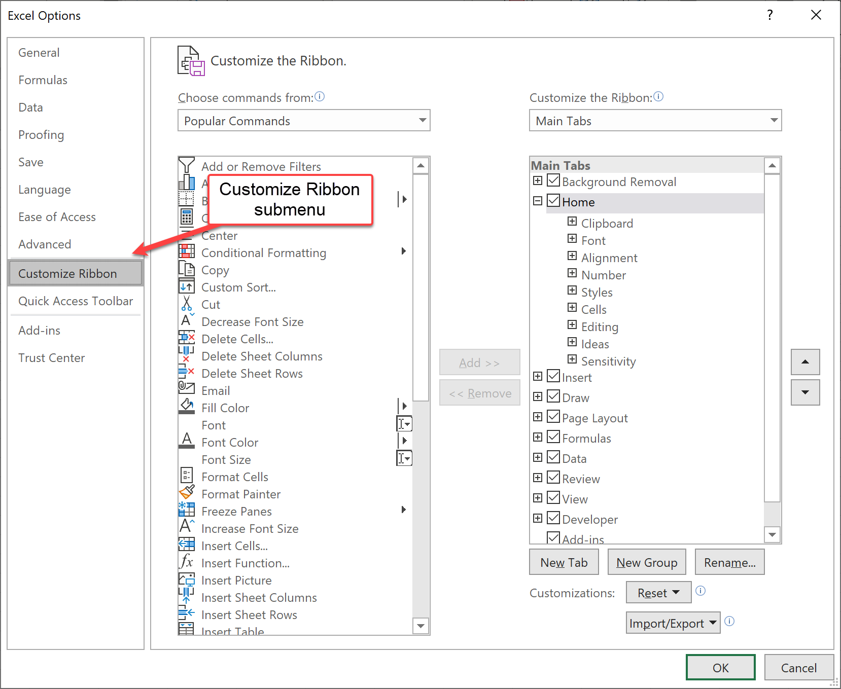
For example, the “Developer” tab is disabled by default. Enabling it gives access to the Visual Basic for Applications (VBA) programming environment.

Another submenu is called Add-ins. Open it. As you can see in the screenshot, this submenu allows you to view and manage plugins for Excel.

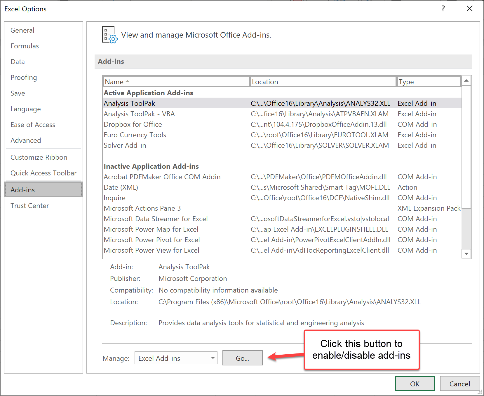
Click on the “Go” button to manage your add-ins.

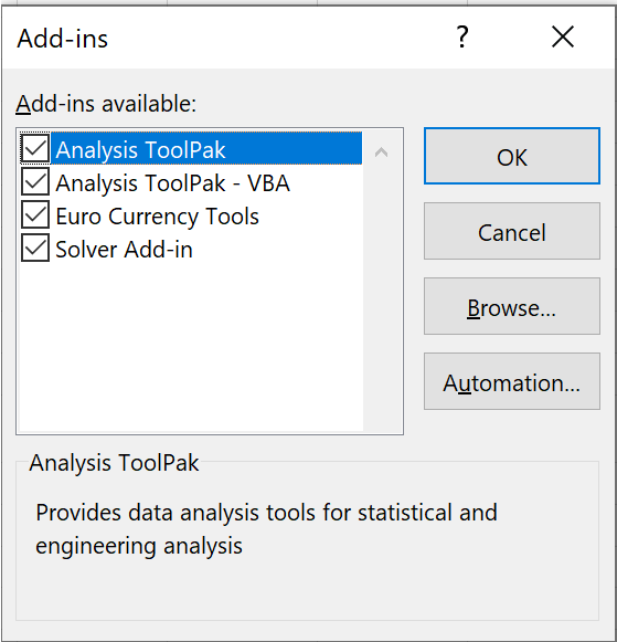
Enable only the add-ins you need. In this tutorial, you will use the Analysis ToolPak (the Data Analysis button in the Data tab). The Solver add-in is also useful later in the course for optimization models. If you cannot enable an add-in, it may not be included in your license or it may be restricted by your IT settings.

Excel has a status bar at the bottom of the screen, which can contain useful information. To illustrate this, put some data in cells A1, A2, and A3, like this:

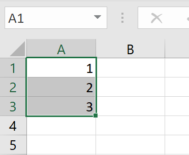
Once you have selected the three cells (as in the screenshot above), some statistics for these cells will appear in the status bar, like Average, Count (= number of selected cells), and Sum:

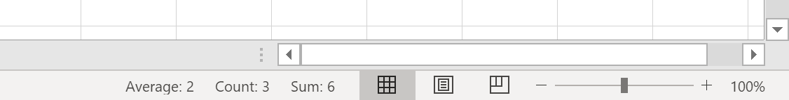
By right-clicking on these statistics, you can customize the status bar. Make sure that Minimum and Maximum are checked. The status bar will then look like this:

This is very useful to quickly get some statistics, without actually having to use formulas, by simply selecting the cells.

Language Settings

Excel can be used in multiple languages. Different languages may use different names. This manual assumes that the English “display language” is used. You can enable these settings under the tab “File”, followed by “Options”, and then the “Language” item (see below).

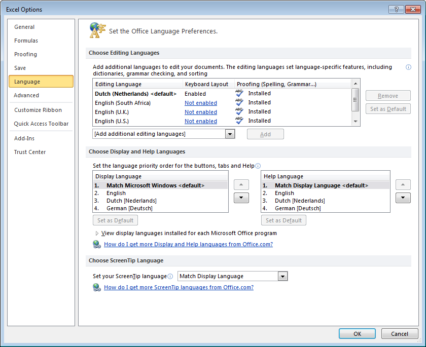
If you do not see the language of your preference in this list, you may add languages via the Microsoft Office Language Preferences (In Dutch: “Taalvoorkeuren voor Office’), which you can find in the Windows start menu. In some cases, your Office license only allows you to use one language.

You may use your own language setting; translation tables for Excel functions can be easily found via Google.

Differences in Formulas Between Countries

Excel uses the regional settings of your operating system. In some countries, a comma (,) is used as a decimal separator, while in others a dot (.) is used. Similarly, the list separator may be a comma or a semicolon (;). This means that formulas may differ between countries.

Therefore, if a formula is not working, perhaps you have to replace commas by semicolons, or vice versa or use a different decimal separator. Since most online resources use the English notation, consider changing your regional settings to English (United States) to avoid confusion.

Excel on a MacBook (MS Office for Mac)

The most recent versions of Excel for Mac contain largely the same features as the MS Windows version of Excel. We highlight some differences here, which may change in future versions, or may already have improved in the version you have.

Keyboard shortcuts on PC and Mac are different. For example, for “Page Up” or “Page Down”, you need to click “FN + Up/Down arrow” on Mac. Some of the shortcuts that work on PC would not work on Mac (for example, “Paste only formulas” or “Paste Link” and others).
Some features differ between Windows and Mac. In some versions of Excel for Mac, PivotCharts and certain add-ins can behave differently. If you cannot insert a PivotChart, create a normal chart based on the PivotTable results, or use Excel for the web/Windows.
VBA has less extensive features on Mac, which only becomes a problem when you are a more advanced programmer.

Excel Version

This tutorial assumes modern Excel (Microsoft 365 / Excel 2021+). If you use an older version, some features (notably XLOOKUP and dynamic arrays) may not be available.

24.3 Assignment: Analyzing Patient Data in Excel

To practice with Excel we will use anonymized data from an operating room department and exercise through various assignments.

80/20 roadmap

If you remember only a few things from this tutorial: keep your data in an Excel Table (CTRL+T), clean/import with Power Query, summarize with PivotTables, look things up with XLOOKUP, and communicate results with a simple chart.

24.3.1 Importing the Data (Patients.xlsx)

To complete the assignments, you need a workbook that contains the two data sheets consultation_history and patient_data.

Recommended: download and open Patients.xlsx.
Alternative (Power Query): rebuild the workbook from the two CSV files below.

If you downloaded the file from a browser, save it to your computer and open it from Excel (not inside the browser). If Excel opens the file in Protected View, click Enable Editing.

What is inside `Patients.xlsx`?

The file contains two worksheets that you will use throughout this tutorial:

consultation_history (≈ 2100 rows, 11 columns): one row per surgery/consultation (includes age, expected duration, registered duration, surgery type, etc.).
patient_data (≈ 2100 rows, 2 columns): patient name and gender.

Column overview:

consultation_history: Patient ID, Week, Day, OR, Gender, Age, Expected duration, Order of surgery, Surgery type, Registered duration, Surgery types
patient_data: Patient name, Gender

Checkpoint (required sheet names)

By the end of the assignments, your workbook should still contain the two original sheets named consultation_history and patient_data. Do not rename these sheets; create additional sheets for calculations, PivotTables, and charts.

Recreate the Workbook from CSV (Power Query) (Optional)

This optional exercise teaches you how to rebuild the workbook from scratch (starting only from raw data files). This is a great 80/20 skill: if you can import and clean data reliably, analysis becomes much easier.

Step 0: Get the two CSV files

These CSV files correspond 1-to-1 to the two worksheets in Patients.xlsx:

Download both files to the same folder on your computer.

Step-by-step (Power Query: CSV -> Excel workbook)

Open Excel and create a new blank workbook.
Go to Data -> Get Data -> From File -> From Text/CSV.
Select consultation_history.csv.
In the import preview, make sure the delimiter is a comma (,). Click Transform Data.
In the Power Query Editor, check:
- Check that the first row is used as headers (Home -> Use First Row as Headers) if needed.
- Verify data types (whole numbers vs decimal numbers vs text). If something looks wrong, click the data type icon in the column header to change it.
- (Optional) Remove blank rows (Home -> Remove Rows -> Remove Blank Rows).
Click Home -> Close & Load -> Close & Load To…
- Choose Table
- Choose New worksheet
Rename the created worksheet to consultation_history.
Repeat steps 2–7 for patient_data.csv (load it as a Table into a new worksheet and rename the sheet to patient_data).
Save your workbook as Patients.xlsx (or Patients_working.xlsx if you want to keep the original Patients.xlsx unchanged).

Checkpoint (your rebuilt workbook)

You should now have a workbook with two worksheets named consultation_history and patient_data. This is the structure the rest of the tutorial assumes.

Microsoft Support:

24.3.2 Quick Navigation

Start on the sheet consultation_history unless an exercise explicitly tells you to use patient_data.

An Excel .xlsx document is called a workbook. Within the workbook are several worksheets (tabs). In this tutorial, the data is stored in the sheets consultation_history and patient_data. A worksheet is a table with numbered rows and alphabetically designated columns. This way, every cell within a table is denoted with a letter-number combination. For example, B3 is the 3rd row, 2nd column.

First, we will edit the screen so that the first row with titles will always be visible when scrolling down. Go to the tab “view”, and press “Freeze panes”. Then press “Freeze top row”. The first row now has a dark underlining and will always stay on the screen even when you scroll down (try this).
When you want to construct a formula, select an empty cell, and type =. When you continue typing, for example, AVE, then a list of commands (these are functions) will pop up starting with AVE.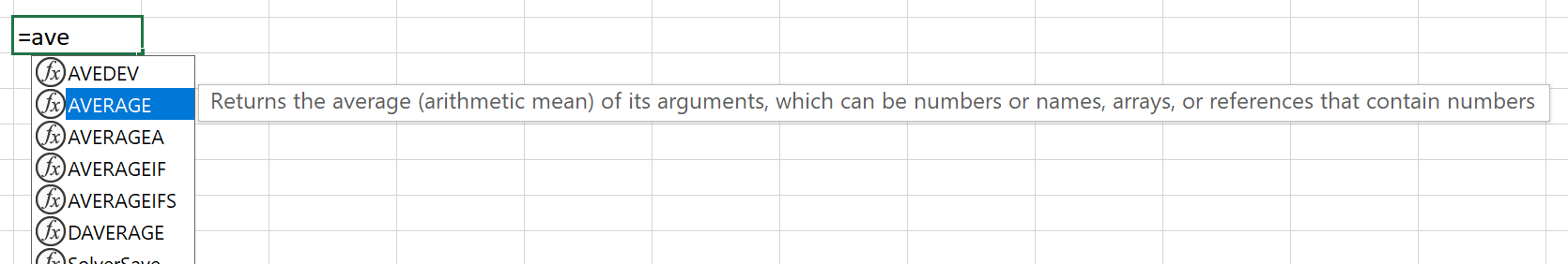

Function Selection

Choose AVERAGE, and press tab. The remainder of the word will be completed by Excel, including the first parenthesis. Now select two cells with numbers, and type ) to close the formula. For example, you now have =AVERAGE(A1:A2). Press enter; the cell now contains the average value of the two selected cells.

HINT: if you forgot to type the closing parenthesis ), Excel will autocomplete it for you, without asking. If parentheses are missing in more complex formulas, Excel will ask you how to complete the missing parentheses.

WarningCase Sensitivity in Excel Formulas

Excel formulas are not case sensitive (i.e., SUM is the same as sum). Excel will automatically format formula names with capitals.
When “creating” formulas, it is a huge time saver to be able to maneuver quickly through a worksheet. Repeat the following steps and observe what happens on screen.
- Select cell A2 (i.e., the first cell with data).
- Press CTRL + ARROW DOWN (to jump to the last cell in the column).
- Press CTRL + ARROW RIGHT (to jump to the last cell in the row).
- Press CTRL + HOME (to jump back to cell A2; note that if you haven’t frozen the top row, it will jump to A1).
- Press CTRL + SHIFT + ARROW DOWN (to select the entire column A2:A2101).
- Press CTRL + SHIFT + ARROW RIGHT (to select all data cells).
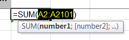
- Go to cell L2 (CTRL + HOME, CTRL + ARROW RIGHT, to quickly go to cell K2, then move to the right).
- Here, type: =SUM(.
- Now press CTRL + HOME. The cell content of cell L2 is now =SUM(A2.
- Now press CTRL + SHIFT + ARROW DOWN. The cell content of cell L2 now is: =SUM(A2:A2101.
- Close the formula: ), and press Enter. Cell L2 has now summed up A2:A2101.
HINT: You can quickly jump to a cell with the “Go To” functionality. Press F5 to use this. For example, jump to cell A1000.

If you were not familiar with these navigation key combinations, train yourself to use them “blindly” by maneuvering through the data as fast as you can (with or without selecting data). Exercise this, as you will experience later that this makes you a lot more efficient.
You can use the mouse to select rows, columns, or ranges of cells.
- Try clicking on a column letter to select that column.
- Try clicking on a row number to select that row.
- Hold CTRL while clicking on column A and then column D. Now you have selected two non-contiguous columns. Of course, this also works on rows.
- Hold SHIFT while clicking on column B and then column E. Now you have selected all (contiguous) columns from B to E.
- Click cell B2. Hold the mouse down, and drag it towards cell E5. Now you have selected all cells {B2,…B5,C2,…,C5,D2,…,D5,E2,…,E5}. In formulas, this is written as B2:E5.

24.3.3 Range and Name

A Range is a collection of cells, for example, A1:A10 (the first 10 cells of column A), or A1:E1 (the first 5 cells in row 1). A range is used in formulas such as: =SUM(A1:A100). When you reference a range on a different worksheet (for example, patient_data), the range is denoted as follows: patient_data!A1:A100.

You can also name a range, in the white space above column A, see the figure. In a new worksheet, enter some numbers in the cells A1 to A3. Select these three cells, and enter in the white space above column A the word UTWENTE. Now place in cell B1 the formula: =SUM(UTWENTE). If you type =SUM( and then press F3, you will see a list with all known ranges to Excel. You should only see the name UTWENTE. Select it, and close the formula with ). Check the result.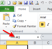

Named Range

24.3.4 Formatting Cells

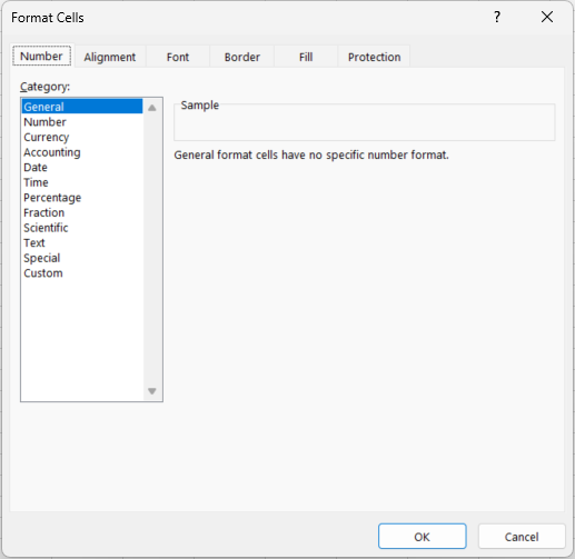
In Excel, data in cells is treated differently depending on the format assigned to the cell. You can assign this using the Format Cells menu (see figure), which you can reach by right-clicking the cell and choosing Format Cells from the menu that appears. Alternatively, press the CTRL + 1 hotkey.

Type the number 3 in a cell and go to the Format Cells menu. When you now select the option Currency from the list on the left, the number 3 is automatically changed to € 3.00. For example, by choosing other options from the list, you can change the number 0.3 to 30% or the numbers 3/1 in 3-1-2010.

In addition, there is also an option Special, which allows data to be formatted as an account number, telephone number, social security number, or place.

Adapting the formatting of the data to the type of data has many advantages. For example, you can avoid unnecessary decimals, make long series of numbers (e.g., telephone numbers) more readable, or automatically show negative amounts of money in red. This increases the readability and clarity of large amounts of data. However, in some situations, there is no standard format for the type of data that you want to process. In that case, you can create your own custom layout (see screenshot).

Type the number 123456789 in an empty cell and press enter. Select the cell and go to the Format Cells menu. Select Custom from the list. In the box to the right, some standard possibilities are given by Excel. When you choose an option from the right-hand box, you will see above it how this option changes the format of your number (try this!). In some cases, however, none of these options is suitable. Suppose a number (serial number, patient ID, process code) starts with a 0, Excel automatically removes this 0. To prevent this, you can create a layout yourself and add it to the Excel options.
Type 0123 in a cell. As soon as you press enter, you see that Excel removes the first 0. Now right-click on the cell and go to the menu Format Cells (shortcut CTRL + 1), the option Custom. The word “standard” appears in the text box under Type. Remove it and replace it with 0000 (four zeros) and click OK. This tells Excel to always fill the number in the cell with zeros up to 4 digits. The number 123 is now supplemented with zeros to 0123, when you type the number 12 this is added to 0012. However, when you type the number 12345, there is no zero because the number already consists of more than 4 numbers. This approach only works if you want all numbers to consist of the same number of digits (for example, with serial numbers).
Suppose you want to let every number start with two zeroes. In this case, you choose (in the text bar under Type) as a format 00###. The #-sign indicates that the original data may hold a digit. In this case, Excel will place two zeroes before every number input that contains at most 3 digits. When you type 1234 in a cell, Excel will change this to 01234. Input data with more than 5 digits will not be changed.
It is also possible to add letters to serial numbers. Suppose all serial numbers consist of an A followed by a maximum of 4 digits. Then use as formatting A000#, and all entered numbers will be completed by zeros up to four digits after the letter A.
In the list of Excel formatting options, you will see that it is also possible to add colors and parentheses. For example, type (000)[Blue] in the Type box, click OK, and type 5 in the cell. You will see that 5 is changed by Excel in (005) in blue.

Should I Memorize All Formatting Options?

It is not expected that you memorize all formatting options. However, you are expected to be able to change the formatting, and if necessary, use online resources to find the desired formatting options (e.g., Google “Excel custom number formats”).

24.3.5 Copy and Paste; Freezing Cell References

Calculate for the expected and the actual operating time the mean and the standard deviation (or the functions AVERAGE and STDEV.P), and place them somewhere at the top of column M or N. Make sure that Excel shows only 1 decimal (decimal). Use the Format Cells menu (shortcut CTRL + 1).

NotePlacing Calculations in Separate Columns

We do not place the mean and standard deviation below the data columns but in a separate column, for a reason. Namely, when there is only data in a column (and no other calculations) you can calculate the average of a column as follows: =AVERAGE(G:G). You do not have to indicate the row numbers! When data is added, you do not have to adjust the formula either, because it applies to the entire column G. However, if you would place the average below the data (e.g., in row 2103) (as follows: =AVERAGE(G2:G2101)), and there are e.g., four rows of data, you first have to insert 4 rows to add the data, and you have to change the formula to =AVERAGE(G2:G2105). That does work, but is not very useful.
With “copy and paste” you can have Excel do many calculations very quickly. It is important here to occasionally make use of the “freezing” of (a part of) the cell range in the formula. We will illustrate that in the next steps:
- Select cell L2, in which we have just calculated the sum of the cells A2:A2101.
- Copy cell L2 (using CTRL + C), and paste it (CTRL + V) to cell M2. Look at the formula in cell M2. This is =SUM(B2:B2101). The formula in L2 was =SUM(A2:A2101). By copying this formula one column to the right (from column L to M), Excel has increased the column-reference to column A by one to B. In other words: in cell M2 the data of column B is added.
- Copy cell L2 (with CTRL + C), and paste it (CTRL + V) in cell L3. Look at the formula in cell L3. This is =SUM(A3:A2102). The formula in L2 was =SUM(A2:A2101). By copying the formula one row down, (from row 2 to 3), Excel has increased the row-references to both row 2 and row 2101 by one, to resp. 3 and 2102. So, in cell L3 we are no longer including cell A2 in the sum, and are now including the (empty) cell A2102! How do we prevent this? This is done by freezing the row references in cell L2 with a $-sign, as follows.
- Change the contents of cell L2 to: =SUM(A$2:A$2101). When you now copy cell L2 to L3, the row references are “frozen’, i.e., are no longer changed (try this!).
- Similarly, column references are frozen by placing a $-sign before the column letter in a reference.
- You can quickly freeze references using the F4 button. Select cell L2, and select the cell-reference A2:A2101 as in the picture:
  
  Freeze References
- Press F4 a number of times, and observe every time what it does with the reference. All variants of freezing cell references with and without $-signs can be obtained this way.
- You can also press F4 immediately after having typed a cell reference in a formula. For example, type the following in cell L2: =SQRT(F2.
- Now press F4, and close the formula with a )-sign, and press Enter.
-Copy cell L2 to L3. The result is the same in both cells: =SQRT($F$2).

24.3.6 Conditional Formatting

To emphasize important data in large spreadsheets you may use Conditional Formatting. It determines the layout of cells based on standard or self-entered rules. To set a formatting rule for a collection of data, first select the data. Then go to the function Conditional Formatting in the Home menu:

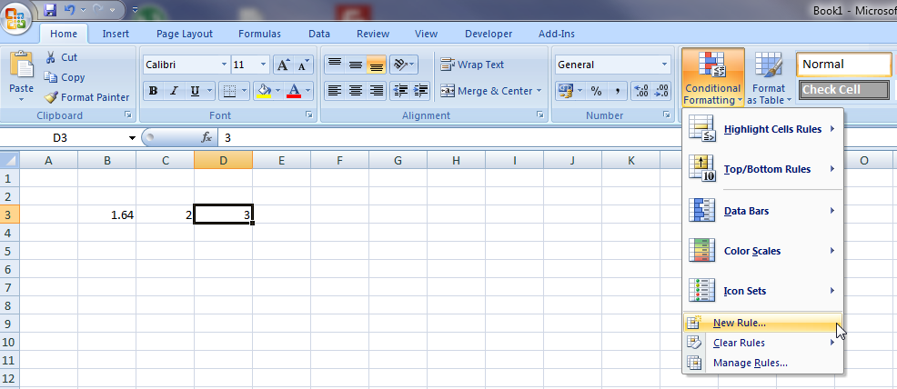
Click on the New Rule option. The New Formatting Rule menu is opened (see figure). Here you can select various options for formatting the data depending on the value. For example, numbers above or below a certain value can be colored. You can also provide all values from the set that are below the average with a specific layout. Even when text is used in the data, you can attach a layout to it. For example, you can color all cells with “yes” green.

Use Conditional Formatting to change the font of all cells in column F with ages “65 and higher” into red and bold.

24.3.7 Autofill

Autofill is a function that allows you to fill cells quickly and automatically with data so that you do not have to do this time-consuming task. Autofill can for example be used to complete a series of numbers, days, or even formulas (like 1, 2, 3, ….). Excel will need at least two starting cells to predict a series of numbers. If you start with 1 and 2, then Excel will predict that the next one should be 3, etc. In the following example, one input is already sufficient.

Open an empty worksheet and write “Monday” in cell B3. (Note: you might have to use the same language as your Excel is in, so in Dutch “maandag”.) We want to place the days of the week next to each other in columns. You can do this by using Autofill:
- Position your cursor on the bottom right corner of cell B3. It will change into a small black + sign.
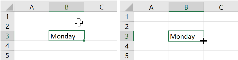
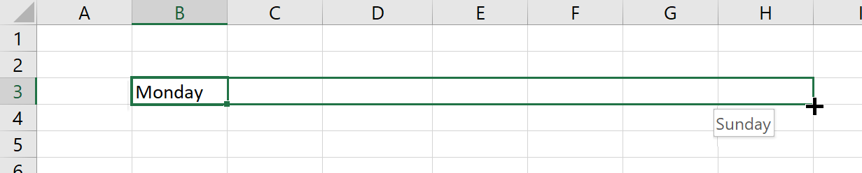
Autofill Handle
- After that, you can click (keep the mouse button pressed down) and drag your cursor to cell H3. Excel will now automatically fill in the correct sequence of days and you can even go beyond cell H3.
  
  Autofill Example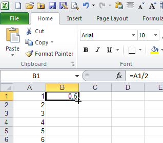
  
  Autofill Results
- Instead of dragging the cells, you can also double-click on the black + sign that appears when you hover your mouse over the bottom right corner of a selected cell. This will autofill all the cells positioned under the original cell up to the row that the previous column was filled.
Fill cells A1:A50 with the numbers 1 to 50 on a new worksheet. Place in cell B1 the formula =A1/2. Double-click the black cross, like in the screenshot. You will see that Excel applies autofill to the cells B2 to B50.
Delete the contents of cell A4 and B4. Put the formula =B1*2 in cell C1. Double-click on the black cross of cell C1. Now you can see that Excel stops to autofill cells when the previous column has an empty cell.

Autofill can also be used for months, years, dates, number series (like 1, 2, 3… or 2, 4, 6…. Or even Patient1, Patient2, ….).

24.3.8 Adjusting Column Width and Row Height

When words or large numbers are put into a single cell, it might occur that the cell is too small resulting in overlapping contents of cells or partly invisible contents. To fix this you can adjust the column width or the row heights of the cells, such that all contents are fully shown. There are two ways to achieve this:

First, select an entire column by clicking on the letter of that column. Then click with your right mouse button on the selected column and choose the option Column Width from the menu. Specify a number to increase the column’s width.
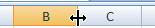
Move your cursor to the top row with the letters of the columns. Position your cursor on the border that two columns share, like in the screenshot. When your cursor changes into a plus sign with horizontal arrow signs, you can click and drag the column to enlarge it. You can also double-click on this special plus sign to “autosize” the column to the minimum required width to show all contents of its cells.

Column Width Adjustment

The exact same principles apply to changing the height of the rows.

If you want to enlarge multiple columns and rows, then you can select them all. When you then click and drag a border to the desirable size, all selected columns and rows will then get that same size. Again, you can also double-click and then the size of all cells will be the same and as large as is needed to show the contents of the largest cell.

Quick Selection of Entire Worksheet

To quickly select the entire worksheet, click on the empty cell in the upper left corner (left of column A and above row 1). Alternatively, you can use the shortcut CTRL + A.

24.3.9 Graphs

To create an overview of how often each surgery type occurs, we want to create a chart that displays the frequencies per surgery type. Excel can display data in various types of charts. A good workflow is:

Create a small summary table (e.g., counts per category).
Select the summary table.
Go to Insert and pick an appropriate chart type.

After you insert a chart, the contextual tabs Chart Design and Format (under Chart Tools) appear. Use these to change the chart type, add chart elements, and format axes/labels.

For more information on charts in Excel, you can watch the following video:

Microsoft also offers some nice examples on chart design.

TIP: In the example above, we first selected the data and then chose a graph type. You can also do it the other way around (first select the graph type, then the data), but this way is usually perceived as much more complex.

Create a column chart (bar chart) that shows the frequency per surgery type. To do so, first calculate the frequencies per surgery type in column Q. You can do this using the COUNTIF function. Fill in the formula in cell Q2 and then use AutoFill to apply the formula to the other rows (up until row 28). To use autofill correctly, you must “lock” parts of the formula as it was explained before.

To be able to estimate the surgery duration, we want to know if there is a relation between the age of the patient and the duration of the surgery.
In a graph (scatter plot/dissemination graph), plot the two different variables against each other. Set the X-axis (horizontal axis) in such a way that only ages between 15 and 85 years are visible. Can a relation be recognized? (hint: add a trend line using the right mouse button menu)? On average, do the surgeries with older people require more time?

24.3.10 Data Analysis ToolPak, Histogram Function

In the following assignments, we will use the Data Analysis ToolPak. This functionality is installed in Excel, however it may not yet be activated and therefore not visible in the ribbon.

If you do not see the Data Analysis button in the Data tab, follow Microsoft Support instructions here: Load the Analysis ToolPak in Excel.

Histogram in Modern Excel

In Microsoft 365 (and Excel 2016+), you can also create a histogram chart directly via Insert → Statistic Chart → Histogram. The ToolPak histogram is still useful when you want a frequency table as output and full control over bin boundaries.

We want to analyze the duration of surgeries in a graph. Make a histogram where in an interval of 10 minutes the frequency is displayed (use the Analysis ToolPak histogram function). When selecting the data (Input and Bin range), do not select the titles, only the data.

24.3.11 IF-Function

The IF function is one of the most used functions. It returns one value if a condition is true, and another value if it is false. Use the following syntax: =IF(logical_test, value_if_true, value_if_false)

(If your Excel uses ; as list separator, replace the commas with semicolons.)

Fill the cells A1 to A10 with arbitrary numbers between 1 and 10. In B1 enter the formula: =IF($A1>=6, "pass", "fail")

In the first part of the formula, the condition is tested (here: whether the value of A1 is larger than or equal to 6). If the condition is met, the formula returns the text "pass", otherwise it returns "fail". Copy this formula to the cells B1 to B10.

If you want an empty cell as output, enter "" into the formula (note: these are two double quotes, not four single quotes!).

IF-functions may also be used within other IF-functions if multiple conditions must be tested. Imagine you have a list of people with 3 columns, name, gender, and age. From this, you want to select all women older than 35. This can be done with the use of a so-called “nested” IF-function (’nested” means a function within a function):

=IF($B2="woman", IF($C2>=35, "woman above 35", "woman below 35"), "man")

An AND-function gives as output “TRUE” when all the conditions are met. When one or more conditions are not met, the output is”FALSE”.

An OR-function returns the text “TRUE” when one of the conditions is met and”FALSE” when none of the conditions is met. The AND-function and OR-function can also be used within an IF-function and combined with other functions.

People aged 65 and above need an extra inspection when they have surgery. We want to flag this in our data.

In the sheet consultation_history, add a new column called Notes and let Excel automatically add the text "extra inspection" for patients aged 65+ (and an empty cell otherwise). Use an IF formula and fill it down for all rows.

We also want to quickly see the surgeries that took longer than 2 hours, with this we can see whether this happens a lot and for which type of surgeries.
Use Conditional Formatting to highlight surgeries that took longer than 2 hours (i.e., Registered duration > 120) in red.

When you made a mistake in a formula and you want to adjust that specific cell, click on the cell and press the F2 key. With the arrow keys, you can then navigate within the formula and correct the mistake.
Try this by going to a cell with a formula and selecting it with a mouse click, then press the F2 key. You will notice that this is a quick and easy way to adjust the cell.

24.3.12 Excel Table

The Excel Table is a very useful functionality of Excel. It makes it easier to manage and analyze data. It also has the advantage that when you add data, all formatting and formulas are automatically applied to the new data. This saves a lot of time. Check the following video about the usability of the Table:

In the sheet consultation_history, convert the data range to an Excel Table (CTRL+T). Name this table Patients.
TipQuick Data Quality Checks
Before you start analyzing, do a few quick checks:
- Are IDs unique? (Conditional Formatting → Highlight Cells Rules → Duplicate Values)
- Are there missing values in key columns? (Filter for blanks, or use COUNTBLANK)
- Are numbers stored as text? (look for green triangles / unexpected alignment)
In the following assignment, we will sort and filter the data. This short Microsoft video focuses on filtering (sorting is in the same area of the ribbon and often used together with filters):
Practice sorting and filtering the Patients table in consultation_history. For example: sort Registered duration (increasing) and filter to show only patients aged 65+.

Approximately a quarter of the patients who had a surgery will be approached for a survey, in connection with research about their pain experience with this organization.
Add a column where automatically and randomly a quarter of the patients will be selected for this survey. You need to do this with the RAND() function, this will select a random number between 0 and 1. Hint: You can do it like this: if RAND() is smaller than 0.25, then select the patients (use the IF() function).

Note: Because you transformed consultation_history into an Excel Table, formulas entered in the first row of a column will automatically fill down to all rows.
The RAND() function recalculates itself every time a cell in a worksheet changes (select an empty cell, press delete; you can see that the cell has another value). Make sure the column does not change by copying it. With the “Paste Special” function, you only select the “values”. You replace the formulas with the calculated values.

The financial administration requires a unique code, which consists of the “Patient ID” and the “Surgery type”.

Add a column that compiles this code (a text field), using the fields “Patient ID” and “Surgery type”. For example, in an Excel Table you can use: =[@[Patient ID]] & "-" & [@[Surgery type]]

24.3.13 Pivot Table

The pivot table (Dutch: “draaitabel”) is a valuable function of Excel. By using pivot tables, data can be analyzed quickly, dynamically, and flexibly. This data can be shown in a table or in a standard graph. First, take a look at this short instruction video:

Now we would like to analyze the consultation data in consultation_history. For this, we will use a pivot table. In the following questions, you have to place each pivot table in a new worksheet, and make sure your calculations are shown with a maximum of 1 decimal. If Excel adds subtotals automatically, remove them (PivotTable Design → Subtotals → Do Not Show Subtotals).

What is the average surgery duration of surgery type NI799 for women? Important: As explained in the instruction video, start by envisioning the pivot table’s rows and columns (i.e., what data fields are needed?), then design it. Here, the data fields needed are Surgery Type, Gender, and Registered Duration. The first two of these should be used for the rows and columns, and the last one to calculate the contents of the table.

WarningKeep Your Pivot Tables Updated

If you change any source data, the pivot tables will not be up-to-date automatically (in contrast to all the other graphics and tables in Excel). Hence, you need to right-click on the pivot table and select the option “Refresh” to update the pivot table.
Take a look at the average surgery duration of women and the surgery type “AF241” in your pivot table. Search in the source data for a woman with surgery type “AF241”, and change the duration of the surgery to 1000 minutes. Note: the average of the pivot table will not change. Right-click on the pivot table for the option “Refresh” to update the average.
What is the average surgery duration for surgery type KG242 for men above 56?
How many hours were spent in total on surgery type WP174 for women?
How many surgeries were done of type IB847 for women?
Which surgery type has the largest average duration? How long is it?
Which surgery has the largest surgery duration standard deviation? And how large is it?
Create a pivot chart from your pivot table, which should show the average surgery duration for each gender and surgery type. Notice that the pivot chart has dropdown items to select a gender or surgery type.

24.3.14 XLOOKUP

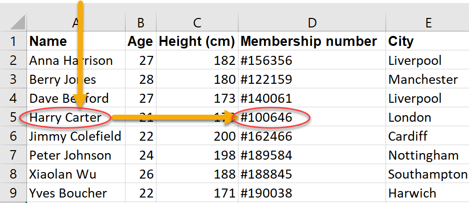
Suppose you want to look up some data in column “Y” of a large table, in the row where there is a particular value in column “X”. For example, say you want the “Membership number” for “Harry Carter” from the table below.

In Microsoft 365 and Excel 2021+, prefer XLOOKUP. Type =XLOOKUP in an empty cell and press F1 to open Excel help for the function.

The function call in the example could be: =XLOOKUP("Harry Carter",$A$2:$A$9,$D$2:$D$9,"Not found")

To find the surgery time of patient number 543 using XLOOKUP, type: =XLOOKUP(543,$A$2:$A$2101,$J$2:$J$2101)

Tip: When you copy formulas down, use $ signs to keep ranges fixed (e.g., $A$2:$A$2101).

No XLOOKUP in your Excel?

If your version of Excel does not have XLOOKUP, use VLOOKUP with an exact match: =VLOOKUP(543,$A$2:$J$2101,10,FALSE)

Give the data of the patient who is 50 years old with AX939, using the AutoFilter function.

24.3.15 Various Functions

Excel has a large number of functions. It is impossible to memorize all of them. However, some functions are used very often, and it is useful to know them by heart. To get an idea of how the functions will work within Excel, you will regularly use the following functions.

SUM, AVERAGE, MEDIAN, MIN, MAX: basic summaries of a range
COUNT, COUNTA, COUNTIF, COUNTIFS: counting (optionally with conditions)
SUMIF, SUMIFS, AVERAGEIF, AVERAGEIFS: conditional aggregation
IF, IFS, AND, OR, IFERROR: logic and error handling
XLOOKUP: look up a value and return the matching result from another column/range
RAND, RANDBETWEEN: random numbers (useful for simulation / sampling exercises)
ROUND, ROUNDDOWN, ROUNDUP, ABS, SQRT, RANK.EQ: common numeric helpers

The following functions are useful for using in formulas:

ROW: retrieve the row number of a cell
COLUMN: retrieve the column number of a cell
INDEX: return a value from a table based on row/column position

The following functions are very useful for editing or creating cells with text:

LEFT: allows you to get a number of characters at the beginning of a text
RIGHT: allows you to get a number of characters at the end of a text
MID: returns characters from the middle of a text
LEN: indicates the length of the text in a cell
&: use this in the formula to link text to each other
TRIM: removes extra spaces
CONCAT / TEXTJOIN: combine texts (older Excel also has CONCATENATE)
TEXT: converts a numeric value to a text
FIND: looks for a text or character in another text
REPT: repeats a character a number of times

Use these functions for the following exercises.

Go to the sheet patient_data, which has a long column with (complete) patient names. Add two columns, and put the first name of the patients in the first, and the last name in the second. HINT: you need the LEN, RIGHT, LEFT, MID, and FIND functions for this.

TipModern shortcut (optional)

In Microsoft 365 / Excel 2021+, you can also split names using Flash Fill (CTRL+E) or TEXTSPLIT(). In this tutorial, we practice text functions to learn how formulas work.
Add a column with “surname, first name” (hint: use the “&” sign to connect two strings together).
Add a column with an arbitrary age of each patient, between 0 and 100 years. Use the RANDBETWEEN function.

Every time you press the F9 button, the ages are re-drawn.
Select the column with ages, and copy them (CTRL + C). Right-click on the same column, and choose “Paste special”, and check the option “values”. The column is now overwritten with the age values. The formulas with RANDBETWEEN in it are now gone, and with F9 no ages are drawn again.
Add a column where the age is indicated as “child” (<18 years), or “adult” (18-64 years), or “65+” (for 65 and over).
Make a table in which you count “child”, “adult”, and “65+”. Use the COUNTIF function for this.
Do the same, but with a pivot table.
A tricky one: calculate the sum of the ages of patients younger than 10 years, but older than 5 years. Do this with the SUMIFS function.

24.3.16 Trace Precedents and Trace Dependents

The “Formulas” tab contains functionality to build and analyze formulas. Very useful are the “trace precedents” and “trace dependents” buttons.

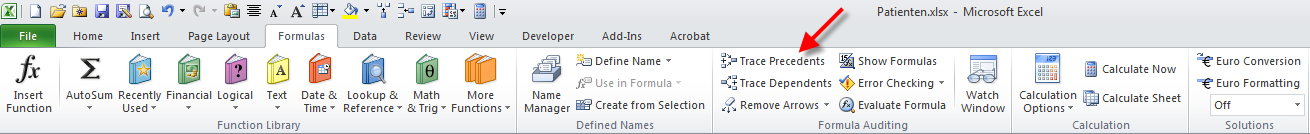
Select a cell that is used in one of the formulas you have just built. Press the Trace Dependents button in the Formulas-tab. You see that arrows appear to all cells using this cell. This allows you to determine whether you can safely erase a cell without changing things elsewhere in the worksheet. Press the Remove Arrows button to remove the arrows again.
Select a cell that contains a formula. Press the Trace Precedents button in the Formulas tab. “Precedent” means predecessor. You see that arrows appear to all cells used in the formula. Press the Remove Arrows button to remove the arrows again.

24.3.17 Data Table

The data table functionality allows you to quickly analyze what happens to the outcome of a calculation when one or two variables you have used in the formula assume different values. As an example, we take the calculation of your Body Mass Index (BMI).

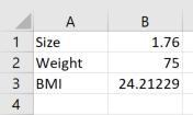
Create a new worksheet, which holds the following data:

In cell B3 there is a formula in which the BMI is calculated as the ratio of Weight and the squared Size (= B2/B1^2). Fill cell E1 with a reference to the cell B3 with the BMI, so with =B3. Fill cells D2:D27 with the numbers 65, 66, ..., 90.

Select the range D1:E27. Go to the Data tab, and under “What-If Analysis” select the “Data Table” option, as shown in the figure:

Data Table

Enter a reference to cell $B$2 (the cell with the Weight) in the “Column input cell” option, and press OK. You see that you have made a table that calculates the BMI for all variants of Weight, with a fixed Size (cell B1).

Write in cell H1 the formula =B3 (or a reference to the BMI formula). In cells H2 to H27, put the numbers 65, 66, ..., 90 again, and in the cells I1 to S1 the numbers 1.70, 1.71, ..., 1.80. Select the range H1:S27, and under “What-If Analysis” select the option Data Table. For Row Input Cell you choose $B$1 (the cell with the Size), and for Column Input Cell you choose $B$2 (the cell with the Weight). Press OK, and view the result.

For a comprehensive explanation of the Data Table with 1 or 2 variables, see: Microsoft Support: Calculate multiple results by using a data table.

24.3.18 Goal Seek

Goal seek allows you to determine what the value for one variable in a formula must be, to retrieve a desired outcome of the formula.

Imagine you want to know how much you should weigh to have a BMI of exactly 25. Click Goal Seek, in the Data tab, under What-If Analysis. You will get this screen:

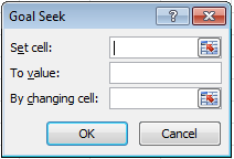
Goal Seek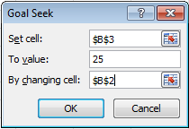

Goal Seek Screen

In the first box, you find an icon. When you click on this icon, you can select the cell in your worksheet where the formula is placed of which you want a certain outcome. Thus, select the cell with the BMI-formula. Type in the second box (“To value”) the number 25, and choose in the last box the cell where the weight is placed (see figure). Click OK. The weight that is calculated is 77.44 (with a size of 1.76). In other words: A weight of 77.44 and a size of 1.76 gives a BMI of exactly 25.

For a more extensive explanation of Goal Seek, see: Microsoft Support: Use Goal Seek to find the result you want by adjusting an input value.

24.3.19 Data Validation

With data validation, you can set conditions for the values allowed in a cell. For example, you can create a dropdown list in each cell containing the appropriate value for that cell. See:

Create a dropdown list in which you can select the surgery type. To do this, first create a list of all surgery types somewhere in your worksheet (for example, in column Z). Then select the cells in the consultation_history sheet where you want to have the dropdown list (for example, column C). Go to the Data tab, and click on Data Validation. In the menu that appears, select under Allow the option List. In the box Source, select the range with all surgery types (for example, =$Z$2:$Z$28). Click OK. Now you can select in each cell of column C the surgery type from a dropdown list.

24.3.20 Printing

Printing is not central to data analysis, but it helps when you need to hand in a worksheet or report.