The Importance Of Using Toy Examples

Richard Feynman, renowned physicist and Nobel laureate, famously said:

“If you can’t explain something to a first-year student, then you haven’t really understood it.”

Toy examples embody this principle: they distill complex models and methods to their essence so the takeaway message gets across quickly and clearly. They are not just simplified versions of a problem; they are carefully crafted illustrations that highlight the core concepts without unnecessary complexity.

A good toy example:

Uses the minimum number of elements. If one dimension suffices, avoid two. If 10 time steps are enough, avoid 100. If two vehicles suffice, avoid three.
Stands alone. Figures must be self-explanatory, with captions and legends allowing comprehension without the main text.
Highlights the gap. The figure should include the element that distinguishes the contribution (new model, algorithm, etc.) from prior work.

Examples From Papers

Below are toy examples taken directly from papers. First, we present the in-text excerpt from where the figure is referenced. Then, we show the figure itself, which is a toy example illustrating the process described in the text.

A Two‑Echelon Multi‑Trip Vehicle Routing Problem With Synchronization For An Integrated Water‑ And Land‑Based Transportation System

Karademir, C., Beirigo, B. A., & Atasoy, B. (2025). A two‑echelon multi‑trip vehicle routing problem with synchronization for an integrated water‑ and land‑based transportation system. European Journal of Operational Research, 322(2), 480–499. https://doi.org/10.1016/j.ejor.2024.10.047

Full In‑Text Excerpt

Figure 1 represents an IWLT network for pickups, multi‑trips by LEFVs, and transfers at satellites executed in synchronization by vessels and LEFVs. All sets, parameters, and decision variables are presented in Table 1.

Figure 1: Example of a small network and a feasible scheduling for the proposed IWLT system, where LEFVs collect goods at the customer level and visit satellites to transship all the goods onto a vessel. A satellite can be visited several times by the same or different vehicles, but at most a vessel and a LEFV perform a transfer operation at a time considering unitary transshipment. This lets vehicles have cycles in space (a) if necessary or efficient while temporal synchronization (b) guarantees that there is no cycle in the temporal‑spatial graph of all operations. For a transfer decision after node \(i\), spatial synchronization is ensured by assigning it to a satellite \(p\) in reach, \(v_{ip}\). Furthermore, the temporal synchronization is ensured by the transshipment start time on a vessel, \(u_i\), without violating time constraints of upstream or downstream operations of the vehicles interacting. Schedules of LEFVs: \(\{x ∶ g \rightarrow 1 \rightarrow 2 \rightarrow 3 \rightarrow 4 \rightarrow 5 \rightarrow 6 \rightarrow g\}\), \(\{x ∶ g \rightarrow 7 \rightarrow 8 \rightarrow 9 \rightarrow 10 \rightarrow 11 \rightarrow 12 \rightarrow 13 \rightarrow g\}\), \(\{\phi∶ 8,3,11,6,13\}\). Schedules of satellites: \(\{v ∶ 8 \rightarrow p_1,3 \rightarrow p_2,11 \rightarrow p_3,6 \rightarrow p_4,13 \rightarrow p_3\}\). Schedule of the vessel: \(\{y ∶ d \rightarrow 8 \rightarrow 3 \rightarrow 11 \rightarrow 6 \rightarrow 13 \rightarrow d\}\).

A Business Class For Autonomous Mobility‑On‑Demand: Modeling Service Quality Contracts In Dynamic Ridesharing Systems

Beirigo, B. A., Negenborn, R. R., Alonso‑Mora, J., & Schulte, F. (2022). A business class for autonomous mobility‑on‑demand: Modeling service quality contracts in dynamic ridesharing systems. Transportation Research Part C: Emerging Technologies, 136, 103520. https://doi.org/10.1016/j.trc.2021.103520

Full In‑Text Excerpt

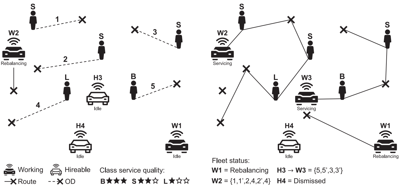
Figure 2 illustrates how a batch of requests from different SQ classes are serviced under this scenario, using a set of working and hireable vehicles. It can be seen from the output sub‑Figure 2 (b) that the high‑SQ class request B5 prompts a hiring operation (\(H3 \rightarrow W3\)) and enjoys a private ride. In contrast, the low‑SQ class request L4 waits longer to be picked up and does not travel directly to its destination (the ride is shared with user S2 momentarily). The working vehicle 2 stops rebalancing to service ODs 1, 2, and 4, whereas candidate vehicle 3 is hired to service ODs 5 and 3. Since working vehicle 1 cannot access any users in time, it repositions to the origin of the hireable vehicle 3 (presumably, an undersupplied region), whereas the idle FAV 4 is dismissed. Therefore, hireable FAVs join the working fleet to help providers honoring service quality contracts by preventing delays and rejections from happening.

Figure 2: (a) The user base is segmented into three classes, namely, business (B), standard (S), and low‑cost (L), which have different expectations towards service quality. The fleet comprises working vehicles (third‑party‑ or company‑owned) and hireable vehicles (third‑party‑owned). (b) To adequately fulfill user expectations across classes, we rely on on‑demand vehicle hiring, inflating the fleet size to avoid service‑level violations.

A Learning‑Based Optimization Approach For Autonomous Ridesharing Platforms With Service‑Level Contracts And On‑Demand Hiring Of Idle Vehicles

Beirigo, B. A., Schulte, F., & Negenborn, R. R. (2022). A learning‑based optimization approach for autonomous ridesharing platforms with service‑level contracts and on‑demand hiring of idle vehicles. Transportation Science, 56(5), 1201–1225. https://doi.org/10.1287/trsc.2021.1069

Full In‑Text Excerpt

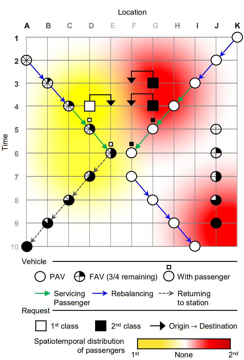
In Figure 3, we illustrate the interplay between the elements of our model. For the sake of simplicity, we represent both vehicle and request discrete locations on a one‑dimensional space for each time step such that \(N = \{A,B,C,D,E,F,G,H,I,J,K\}, \qquad T = \{1,2,\dots,10\}\). We assume it takes a single period to travel between each location pair.

We represent the stochastic process \(F_P\) in time and space by manipulating the transparency of yellow and red colors, corresponding to first‑ and second‑class customers, respectively (see the color bar at the bottom). Regardless of the class, the more opaque is the color, the higher is the probability of finding a request. We assume first‑class requests (i) generate higher profits, and (ii) demand higher service levels, such that failing to adhere to their performance requirements incur higher penalties. We illustrate such higher service levels by assuming first‑class users require to be picked up within one period, whereas second‑class users are willing to wait up to two periods. In turn, regarding the availability of the freelance fleet, we represent the stochastic process \(F_O\) using the shades of gray on the axis tick labels. We assume that the darker is the shade, the higher is the chance of an FAV appearing. Additionally, we assume FAV contract durations last on average four time steps.

In the following, we describe the behavior of three vehicles in detail throughout ten periods. First, at time \(t = 1\), the PAV at location K is faced with two decisions; namely, it can stay in its current location or move to a more promising location in anticipation of future demand. Promising areas consist of high‑demand locations that typically generate the highest profits to the service provider. Pursuing such future profits, the PAV performs two rebalance movements, moving empty from K to J, and from J to I. Once it arrives at location I at time \(t = 3\), the PAV is assigned to a second‑class request (black square) demanding a trip from G to F (solid upper arrow). From this moment on, we consider the PAV is servicing the user, which covers both pick‑up and delivery times. Once the PAV delivers the second‑class user at F, it stays in F for one period, and then rebalances to location I, in anticipation of future passenger demand.

Second, at decision time \(t = 2\), an FAV with an eight‑period contract duration becomes available at location A and is immediately rebalanced to the high‑demand area. Upon arriving at location C, it is matched to a first‑class request demanding a trip from D to E. The FAV travels from C to D to pick up the user and finishes the service at location E and time \(t = 6\). By this time, the FAV is available for four additional periods but spends this remaining time traveling back to its station at A to comply with the contract deadline.

Finally, at location J and time \(t = 5\), a second FAV with a four‑period contract duration appears. However, since it cannot reach high‑demanding areas in the subsequent periods, this vehicle ends up not being hired by the platform, staying still until the end of its contract at time \(t = 9\).

To Wait Or Not To Wait? A Learning‑Based Approach For On‑Demand Ride‑Pooling Water Transport Systems

Beirigo, B. A., & Atasoy, B. (2022). To wait or not to wait? A learning‑based approach for on‑demand ride‑pooling water transport systems. INFORMS Transportation Science and Logistics (TSL) 2022 Extended Abstracts.

Full In‑Text Excerpt

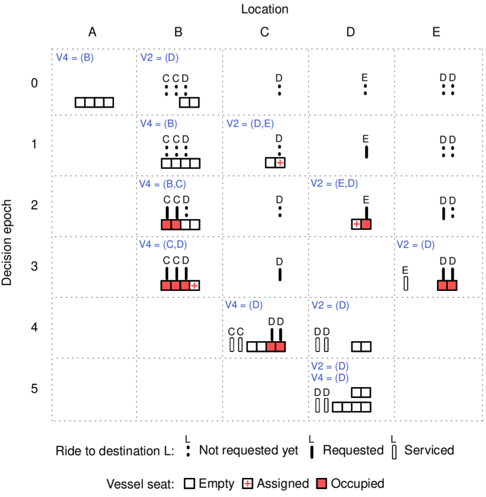
Figure 4 illustrates how an on‑demand ride‑pooling water transport system can harness anticipatory decision‑making to improve service levels. We consider two vessels, V2 and V4, of capacity two and four, respectively, operating on a one‑dimensional service area comprised of five dock locations \(l = \{A,B,C,D,E\}\). These vessels are required to service pickup‑delivery request list \(R = \{B-C,B-C,B-D,C-D,D-E,E-D,E-D\}\) appearing throughout decision epochs \(t = \{0,1,3,4,5\}\). Vessels and requests depicted across locations at each decision epoch \(t\) represent the post‑decision state of the system at \(t\), that is, the state resulting from the decisions taken based on information arriving between epochs \(t-1\) and \(t\). Each request can be represented at three stages: (i) not requested yet, (ii) requested, and (iii) serviced. Requests at stage (i) are uncertain but may be forecasted by the system. As soon as a request appears, it can be assigned to a vessel seat, therefore entering the vessel’s route plan (upper left tuple) featuring the next locations to visit.

By taking advantage of requests’ stochastic information, at \(t = 1\), V4 rebalances to B, and V2 rebalances to D. Passengers at locations B and D are yet to appear, but the system anticipatorily routes vehicles to these locations such that they can promptly service requests as soon as they emerge. The rebalancing route plan is also motivated by the vessel sizes: V2 could not adequately fulfill the demand expected at B, being better suited for the demand forecasted at C, D, or E.

Later, at \(t = 1\), V4 waits at B, whereas V2 is matched to a request from D to E that appeared between \(t = 0\) and \(t = 1\). At \(t = 2\), two B‑C requests are picked up by V4, which updates its plan to add destination C, but delays its departure, expecting to accommodate predicted requests at B. In the meantime, V2 picks up request D‑E and is matched to an E‑D request.

Subsequently, at \(t = 3\), requests B‑D, C‑D, and E‑D appear. Then, at \(t = 3\), while V4 picks up B‑D and is assigned to pick up C‑D, V2 drops off a user at E and picks up two E‑D requests. Next, at \(t = 4\), V4 delivers two users and picks up the previously matched request C‑D, whereas V2 drops off all its passengers. Finally, at \(t = 5\), both vessels are completely unoccupied and plan to wait at location D.

Figure 4: Example of an on‑demand ride‑pooling water transport system working on a one‑dimensional service area throughout time. Besides picking up riders, the two‑seat vehicle V2 and the four‑seat vehicle V4 may wait (empty or not) at their current locations or rebalance to different locations in anticipation of future demand.

Integrating People And Freight Transportation Using Shared Autonomous Vehicles With Compartments

Beirigo, B. A., Schulte, F., & Negenborn, R. R. (2018). Integrating people and freight transportation using shared autonomous vehicles with compartments. IFAC‑PapersOnLine, 51(9), 392–397. https://doi.org/10.1016/j.ifacol.2018.07.064

Full In‑Text Excerpt

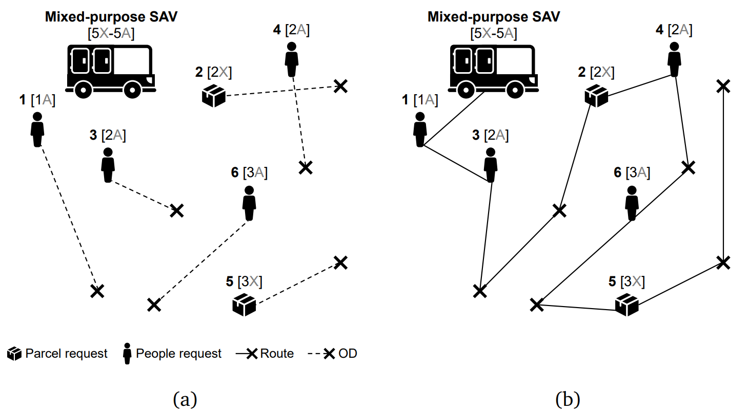
Figure 5‑a) highlights the differences from Li et al. [55] implementation, making explicit the concept of compartmentalized requests. A mixed‑purpose SAV comprised of five compartments of type “A” and five compartments of type “X” (represented as 5X‑5A) is supposed to find the best route to service a set of six transportation requests (two parcels and four people). Besides the identification number, each request also includes, between brackets, the number of compartments of each type demanded. Figure 5‑b) shows the resulting route from the problem presented in Figure 5‑a). The occupancy status of the vehicle after visiting each point (in terms of available compartments) is given by the sequence {1: 5X-4A, 3: 5X-1A, 1’: 5X-4A, 3’ : 5X-5A, 2: 3X-5A, 4: 3X-3A, 4’ : 3X-5A, 6: 3X-2A, 6’ : 3X-5A, 5: 0X-5A, 5’ : 3X-5A, 2’ : 5X-5A}. Assuming request IDs also indicate their order of appearance, one should notice that the ridesharing route presented in Figure 5‑b) privileges people demands, occasionally postponing parcel demands.

Figure 5: Example of a PFIT system. (a) A mixed‑purpose capacitated SAV must fulfill both people and parcel requests. (b) Both request types are integrated into the same vehicle throughout the route.