7  Warehouse Storage: Layout and Space Allocation

Keywords

Warehouse Design, Storage Assignment, Lane Depth, Forward Area, Cross-Docking, EOQ, MIP

A place for everything, and everything in its place—Benjamin Franklin

Learning Objectives

• Differentiate the function of the main warehouse areas and the flows that connect them.
  
• Evaluate lane-depth choices and explain honeycombing and FIFO implications.
  
• Configure a forward area by balancing pick savings and replenishment costs.
  
• Derive EOQ-based dwell time and use it to parameterize space and cost terms.
  
• Formulate and solve a joint SKU-to-flow and area-sizing problem with a clear objective and constraints.

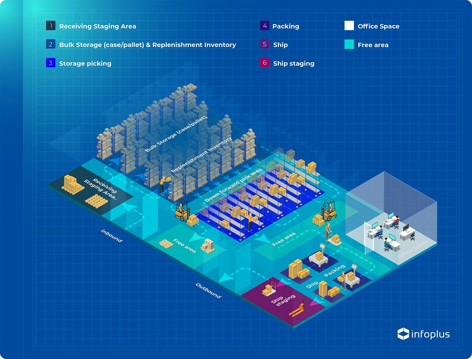
7.1 Warehouse Functional Areas

Warehouses are organized into key functional areas to optimize operations:

• Receiving: Processes incoming pallet loads or cartons, staging them briefly (if needed) before routing to cross-docking, reserve, or forward areas.
• Cross-docking: Sorts and consolidates pre-sorted supplier items for immediate shipping, either directly or after brief staging.
• Reserve (Bulk/Unit-Load Storage): Stores bulky items for extended periods using high-density equipment to maximize space efficiency, with minimal value-added operations.
• Forward (Fast/Primary Picking): Compact area for rapid picking, value-added operations (e.g., labeling, kitting), and order collation.
• Shipping: Prepares picked items (e.g., shrink-wrapped, packed) and stages them for outbound transport.

As shown in Figure 7.1, cross-docking and reserve areas are typically near the shipping dock, while the forward area is close to picking aisles for efficiency.

Figure 7.1: Warehouse functional areas (source)

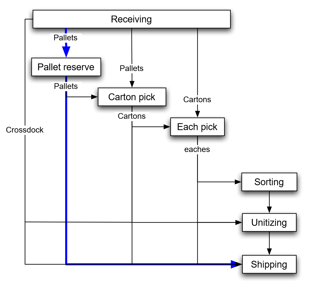
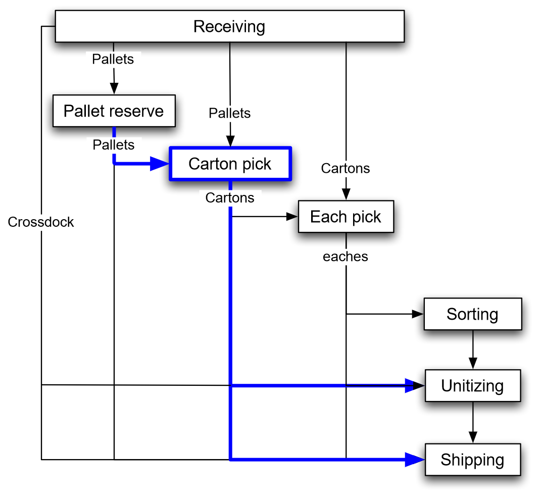
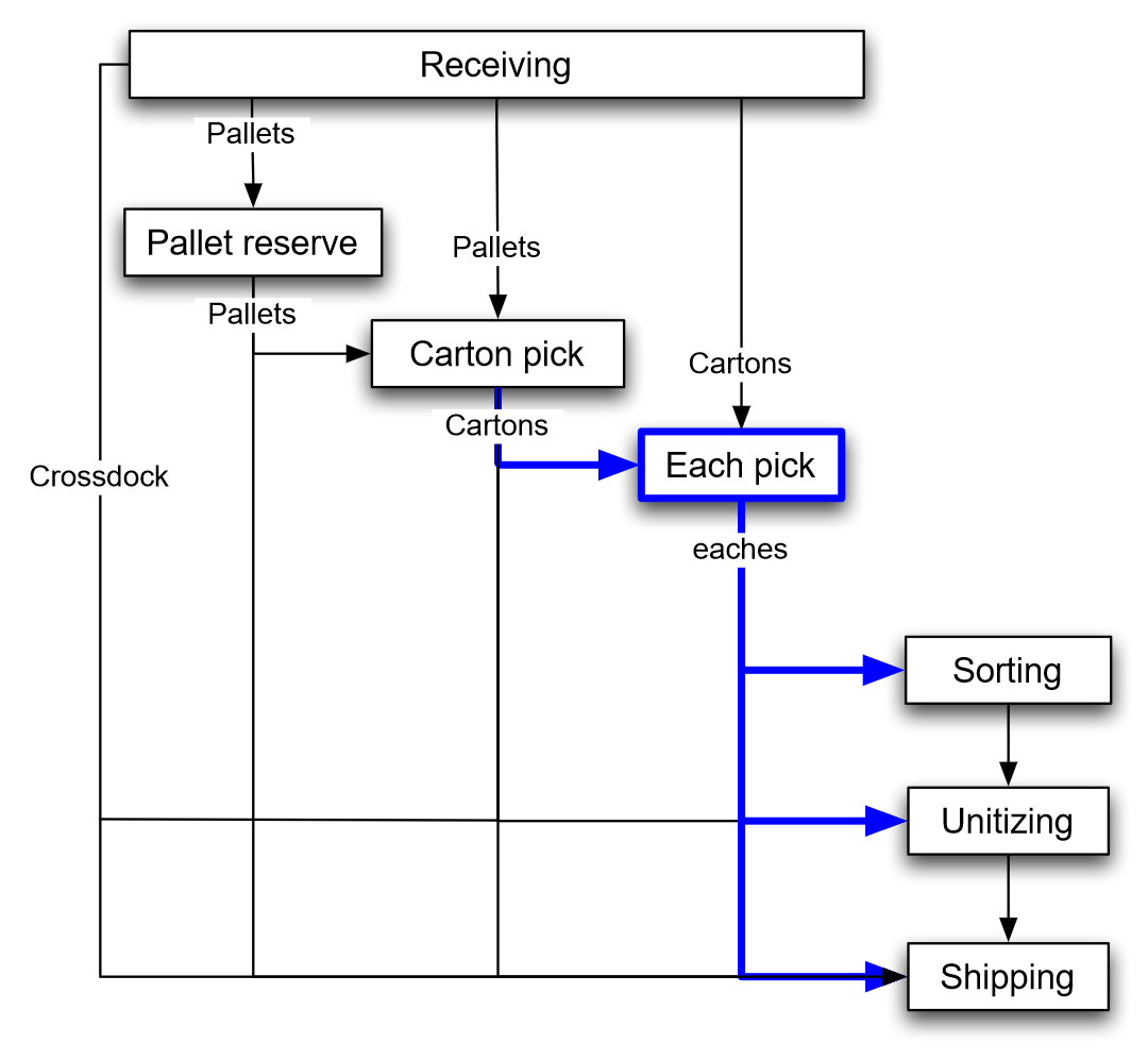
7.2 Material Flows

Figure 7.2 illustrates the flow of unit-loads, cartons, and products through a warehouse:

1. Receiving → Cross-docking → Shipping
2. Receiving → Reserve → Shipping
3. Receiving → Reserve → Forward → Shipping
4. Receiving → Forward → Shipping

(a) Flow of unit-loads

(b) Flow of cartons

(c) Flow of product through piece picking

Figure 7.2: Material flows in a typical warehouse (Bartholdi and Hackman 2019).

7.3 Reserve (Bulk/Unit-Load) Storage

Unit-loads (e.g., pallets) are a significant focus in many warehouses. Per Bartholdi and Hackman (2019), space and labor needs scale linearly with the number of units handled.

A key question is:

How can space cost-efficiency (pallet positions¹ per unit area²) be improved?

Unused space reduces efficiency and increases costs. Two strategies are:

• Maximize vertical space: Taller racks increase pallet storage within the same footprint but may require specialized equipment (e.g., high-reach forklifts or AS/RS) and more labor for retrieval.
• Use deeper lanes: Store more pallets per aisle, but this can reduce accessibility, complicate FIFO retrieval, and increase honeycombing³.

“The simplest type of warehouse is a unit-load warehouse, which means that only a single, common “unit” of material is handled at a time. The typical unit-load is a pallet. Because pallets are (mostly) standardized and are (mostly) handled one-at-atime, both space and labor requirements scale: It takes about n times the space to store n pallets as for one; and it takes about n times the labor to handle n pallets as for one. An example of unit-load is a 3rd party transshipment warehouse that receives, stores, and forwards pallets. The 3rd party warehouse is a subcontractor to others for warehouse services. A 3rd party warehouse typically charges its customers for each pallet handled (received and later shipped); and rent for space occupied. In this chapter we study unit-load issues in the context of such a warehouse; but many warehouses have some portion of their activity devoted to moving unit-loads, as in Figure 6.1.” (John J. Bartholdi and Steven T. Hackman, 2019, p. 51) (pdf)y

“One revenue source of the 3rd party warehouse is to charge rent by the pallet-month. But because the warehouse typically tallies its own expenses by the square-foot or square-meter (for example, rent of the building, climate control, cleaning, and so on), the warehouse naturally wants many pallet-positions per unit area. It can achieve this in two ways: by taking advantage of vertical space and by using deep lanes.” (John J. Bartholdi and Steven T. Hackman, 2019, p. 51) (pdf)

7.3.1 Optimal Lane Depth

Aisles provide accessibility rather than storage. Deeper lanes amortize aisle space across more pallet positions but reduce accessibility and FIFO compliance. With dedicated storage, interior positions may remain unavailable to other SKUs after the first extraction. This waste is honeycombing. The design task is to pick a lane depth that minimizes unoccupied floor space-time that is not reusable by other SKUs (Bartholdi and Hackman 2019).

Hence, the choice of lane depth involves trade-offs between space utilization and operational efficiency.

Shallow lanes:

• More space lost in aisles.
• Increased accessibility.
• Faster position reassignment.

Deep lanes:

• More space for pallet positions.
• Reduced compliance with FIFO.
• Increased S/R times.

For example, pallet position (p.p.) engagement (see Figure 7.3) varies by lane depth:

• 1-deep: 8 aisles, 196 directly accessible p.p’s.
• 2-deep: 6 aisles, 140 directly accessible p.p’s.

A pallet position, consists of the footprint of the pallet plus any required clearance space.

(a) 1-deep lane depth (8 aisles and 196 pallet positions)

(b) 2-deep lane depth (6 aisles and 280 pallet positions, of which 140 are directly accessible)

Figure 7.3: The 2-deep layout fits 84 (42.86%) more pallet positions than the 1-deep layout. However, it may lead to increased handling times and reduced accessibility for certain SKUs.

“Lane depth

Aisles provide accessibility, not storage, and so this space for aisles is not directly revenue-generating. Consequently we prefer to reduce aisle space to the minimum necessary to provide adequate accessibility. For this the aisles must be at least wide enough for a forklift to insert or extract a pallet. By storing product in lanes, additional pallet positions can share the same aisle space and so amortize that cost. Should lanes be four pallets deep? Six? Ten? There are many issues to consider, but the most important one is effective utilization of space. For example, double-deep layout (lanes that are two pallet-positions deep) fits about 41% more pallet positions in the same floor area than does single-deep layout in the example of Figure 6.3; but is it a better layout? Are enough of the additional pallet positions usefully engaged? There is a trade-off: The single-deep layout has eight aisles and provides 196 pallet storage locations, all of which are directly accessible, which means that they are available for reassignment as soon as the current pallet is shipped out. In contrast, the double-deep layout has only six aisles and provides 280 pallet storage locations—but only 140 of them are directly accessible. Moreover, the 140 that are directly accessible are not available for reuse until the interior pallet location in the same lane becomes available. So: Deeper lanes produce more pallet storage locations but they are of diminishing value. By pallet position we mean the floor space required to hold a pallet. This includes not only the footprint of the pallet but also any required gap between one pallet and an adjacent one (Figure 6.4). Let the lanes be k pallet positions deep. Each lane requires aisle space at its head so that pallets can be inserted and removed.

Page 77 2023-05-29#5:41 am

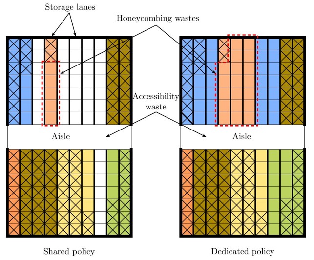
7.3.2 Lane Depth and Storage Policies

Besides space utilization, lane depth also impacts storage policies. Different policies can be adopted based on the lane depth and the specific requirements of the warehouse operation.

Dedicated Policy. In some industries, a dedicated storage policy is employed, where specific SKUs are assigned to specific locations within the warehouse. This approach can enhance picking efficiency and reduce search times. However, it may lead to poor space utilization, especially in deep lanes, as a larger share of unoccupied interior locations may become unavailable to other SKUs after a retrieval (honeycombing).

Randomized (Shared) Policy. In contrast, a randomized or shared storage policy allows multiple SKUs to share the same storage locations. As pointed out by Derhami, Smith, and Gue (2017), this policy can be operated with allowing blockage (i.e., permitting different SKUs to occupy the same lane) or without allowing blockage (i.e., each lane can only hold a single SKU). The choice must consider the specific operational requirements and constraints of the warehouse:

• Inventory/SKU is Low -> Allow Blockage. Allowing blockage can be beneficial in situations where there is a high variety of SKUs but low inventory levels. This approach enables more efficient use of space by allowing different SKUs to share the same lane, thus minimizing the risk of unoccupied pallet positions. The goal shifts towards maximizing the utilization of available space while minimizing the costs associated with relocation and reorganization.
• Inventory/SKU is High -> No Blockage. In contrast, a no-blockage policy may be more appropriate when there is enough inventory to justify dedicating a lane to a single SKU. In this case, to avoid blockage and relocation, a lane is dedicated to a SKU once it occupies the first position of the lane. Honeycombing is more pronounced in this scenario, as unoccupied positions within the lane may remain inaccessible to other SKUs until the dedicated SKU is fully retrieved.

“The shared policy is operated with allowing or not allowing blockage. When the variety of SKUs is large but their inventory is small, assigning a lane to a single SKU is not justifiable, and therefore, different SKUs have to be stored in the same lane. In this case, blockage is inevitable and the goal is to arrange SKUs such that the relocation costs are minimised. An example of such a case is the storage space allocation problem in a marine container terminal (Yang and Kim 2006; Jang, Kim, and Kim 2013; Petering and Hussein 2013; Carlo, Vis, and Roodbergen 2014). On the other hand, when the inventories of the SKUs are big enough to justify assigning a lane to a single SKU, no blockage policy is enforced. In this case, to avoid blockage and relocation, a lane is dedicated to a SKU once it occupies the first position of the lane. This case mainly occurs in the warehouses located in manufacturing systems or the distribution centres where plenty of pallets of different SKUs are block-stacked. However, this restriction wastes storage spaces in a lane when it is filled or depleted as there will be some unoccupied pallet positions in the lane that are just available to the pallets of the assigned SKU.” (Derhami et al., 2017, p. 6436) (pdf)

“This effect is termed honeycombing and waste associated with it is incurred to the system until a lane becomes entirely occupied or empty (Hudock 1998). In addition to honeycombing, aisles also contribute to the overall wasted space. Aisles are required to have access to the lanes but their devoted spaces are not directly used for storage. Warehouse designers aim to minimise these two types of waste to enhance space utilisation in the warehouse. The following example shows how waste of storage space is calculated in a lane.” (Derhami et al., 2017, p. 6437) (pdf)

Figure 7.4 illustrates the differences between dedicated and randomized storage policies in the context of lane depth considering a block stacking warehouse. A block stacking warehouse is a type of unit-load warehouse employing a storage system where pallets are stacked on top of each other, typically without the use of racks.

The optimal lane depth minimizes floor space-time that is unoccupied but unavailable to other SKUs.

Figure 7.4: Honeycombing effect in dedicated and shared storage policies in a block stacking warehouse where lanes are assigned to specific SKUs (no-blockage). Squares indicate a pallete position and squares marked with an “X” indicate occupied positions (source)

“In laying out pallet storage there are other issues to consider besides space utilization. For example, in some warehouses, such as those of food distributors, it is important to move product in accordance with the rule of “First In First Out” (FIFO). Some special types of rack such as pallet flow rack support FIFO; but otherwise FIFO can be guaranteed only to within the lane depth. Making lanes deeper might give better space utilization; but it reduces compliance with FIFO. In addition, deeper lanes can increase insert/extract times.” (John J. Bartholdi and Steven T. Hackman, 2019, p. 69) (pdf) FIFO

A conceptual characterization of the problem: More shallow lanes imply more of them, and therefore, more space is lost in aisles (the size of which is typically determined by the maneuvering requirements of the warehouse vehicles) On the other hand, assuming that a lane can be occupied only by loads of the same SKU, a deeper lane will have many of its locations utilized over a smaller fraction of time (“honeycombing”). So, we need to compute an optimal lane depth, that balances out the two opposite effects identified above, and minimizes the average floor space required for storing all SKU’s. Lanes Lane Depth (3-deep) Lane Height Aisle

“Lane depth Aisles provide accessibility, not storage, and so this space for aisles is not directly revenue-generating. Consequently we prefer to reduce aisle space to the minimum necessary to provide adequate accessibility. For this the aisles must be at least wide enough for a forklift to insert or extract a pallet. By storing product in lanes, additional pallet positions can share the same aisle space and so amortize that cost. Should lanes be four pallets deep? Six? Ten? There are many issues to consider, but the most important one is effective utilization of space. For example, double-deep layout (lanes that are two pallet-positions deep) fits about 41% more pallet positions in the same floor area than does single-deep layout in the example of Figure 6.3; but is it a better layout? Are enough of the additional pallet positions usefully engaged? There is a trade-off: The single-deep layout has eight aisles and provides 196 pallet storage locations, all of which are directly accessible, which means that they are available for reassignment as soon as the current pallet is shipped out. In contrast, the double-deep layout has only six aisles and provides 280 pallet storage locations—but only 140 of them are directly accessible. Moreover, the 140 that are directly accessible are not available for reuse until the interior pallet location in the same lane becomes available. So: Deeper lanes produce more pallet storage locations but they are of diminishing value. By pallet position we mean the floor space required to hold a pallet. This includes not only the footprint of the pallet but also any required gap between one pallet and an adjacent one (Figure 6.4). Let the lanes be k pallet positions deep. Each lane requires aisle space at its head so that pallets can be inserted and removed. Let the aisle space in front of the pallet be of area a, measured in pallet positions. Then the total area charged to one lane is k + a/2 pallet positions. This area is the sum of space devoted to storage (k) and space that provides accessibility (a/2). In most warehouses a lane is dedicated entirely to a single SKU to avoid doublehandling pallets. This saves time but incurs a cost in space: When the first pallet is retrieved from a lane, that position is unoccupied but unavailable to other SKUs. The deeper the lane, the greater this cost. The first pallet position in a k-deep lane that holds uniformly moving product will be occupied only 1/k of the time, the second 2/k of the time, and so on (Figure 6.4). This waste is called honeycombing. Deeper lanes are more susceptible to honeycombing; but shallow lanes use more space for accessibility. Table 6.1 displays daily snapshots of a SKU with an order size that occupies four pallet positions and which is extracted at a rate of one pallet-position per day. In singledeep rack, all the unused space is the aisle space required for accessibility. Deeper aisles require less aisle space per pallet position — but the additional pallet positions are less fully occupied. To maximize space efficiency SKU i should be stored in a lane of depth that minimizes floor space-time that is unoccupied but unavailable to other SKUs. The optimum lane depth can be determined by simply evaluating all possibilities, as has been done in Table 6.1. In Figure 6.5 waste has been plotted for each lane depth, and it can be seen that 2-deep lanes are most space efficient when the aisle is less than 4 pallet positions wide; otherwise 4-deep is best.” (John J. Bartholdi and Steven T. Hackman, 2019, p. 54) (pdf)

7.3.3 Lane Depth and Storage Equipment

The choice of lane depth also influences the selection of storage equipment. Different equipment types are suited to varying lane depths and operational requirements:

• Selective Pallet Racking: Ideal for shallow lanes (1-2 deep), offering direct access to each pallet. It is flexible and allows for easy reconfiguration but may not maximize space utilization.
• Double-Deep Racking: Suitable for medium lane depths (2-4 deep), providing a balance between accessibility and space efficiency. It requires specialized forklifts for accessing the second pallet.
• Drive-In/Drive-Through Racking: Best for deep lanes (4+ deep), maximizing storage density. However, it limits accessibility and may complicate FIFO compliance.

The choice of storage equipment should align with the warehouse’s operational goals, SKU characteristics, and handling requirements.

7.3.4 Aisle Width, Lane Depth, and Material Handling Equipment

As pointed out by Bartholdi and Hackman (2019), aisle space is not directly revenue-generating, so minimizing aisle width is desirable. However, the aisle must be wide enough to accommodate the material handling equipment (MHE) used in the warehouse.

Figure 7.5 illustrates how decreasing aisle width to 1 can lead to significant space savings, leading to 336 pallet positions, which is 140 (71.43%) more than the 1-deep layout (see Figure 7.3 (a)) with an aisle width of 3, and 56 (20.00%) more than the 2-deep layout (see Figure 7.3 (b)) with an aisle width of 3.

Figure 7.5: Warehouse layout with narrow aisles. More space is available for storage.

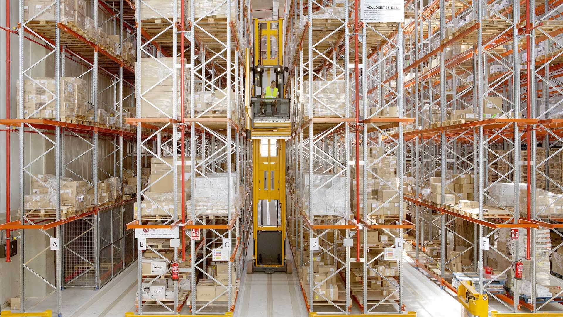
Ultimately, the aisle size and space savings is a compromise between the MHE requirements and costs, and the space savings achieved by narrower aisles. For example, Very Narrow Aisle (VNA) forklifts can operate in aisles as narrow as 1.5 meters (see, e.g., Figure 7.6), significantly reducing aisle width and increasing storage density. However, they require specialized training and may have higher acquisition and maintenance costs.

Figure 7.6: Example of VNA forklift (ArRacking Storage Solutions).

Lane depth will also influence the choice of MHE. For instance, deeper lanes may require specialized forklifts or automated systems to access pallets stored further back in the lane. For example, reach trucks or drive-in/drive-through racking systems may be necessary for deeper lanes.

7.3.5 Optimal Lane Depth for Block Stacking

Block stacking involves storing pallets of a single Stock Keeping Unit (SKU) in floor lanes, stacked to a fixed height, and accessed from one side. This method is commonly used for high-density storage, where pallets are organized in multiple bays of lanes separated by aisles to optimize space utilization and accessibility. However, two primary sources of space inefficiency arise in this system:

1. honeycombing waste within lanes and
2. accessibility waste for aisles that provide access.

Figure 7.7: Block stacking is a common practice in beverage and food warehouses.

Problem Description

In this context, the optimal lane depth problem can be described as follows:

• SKUs are stored in lanes of fixed depth.
• Lanes are last-in first-out (LIFO) (i.e., the most recently added pallet is the first to be removed).
• Lanes are accessible from one side (i.e., the front).
• Batch arrivals are deterministic (i.e., known arrival times and quantities).
• Batch arrivals are either:
  • instantaneous (i.e., all pallets arrive at once), or
  • at finite rate (i.e., pallets arrive over time).

Goal: Determine the optimal common lane depth that minimizes average space waste across all SKUs. Average space waste is defined as the combined impact of honeycombing (unoccupied but unavailable pallet positions) and aisle accessibility waste (space devoted to aisles rather than storage).

Typical Problem Formulation

Let \(N\) be the number of SKUs. For each SKU \(i \in \{1,\dots,N\}\):

• \(Q_i\): batch size in pallets.
• \(P_i\): production or storage rate in pallets per hour.
• \(\lambda_i\): depletion or demand rate in pallets per hour.
• \(Z_i\): stack height in pallets.
• \(A\): aisle width in pallet units.
• \(Z_i*x_c\): total lane depth in pallet units, where \(x_c\) is the common lane depth to be determined.

Objective. Determine the optimal common lane depth \(x_c^*\) that minimizes the total average space waste across all SKUs.

Common Approaches

Several approaches have been proposed to determine the optimal lane depth. Notably:

• Analytical Models. Models that focus on deriving closed-form solutions or heuristics for optimal lane depth. Typically, classical models (see, e.g., Matson 1982; Kind 1975) assume:

  1. Dedicated storage policy, where each SKU is assigned its own lane.
  2. Deterministic and instantaneous batch arrivals.

  Recent advancements (e.g., Derhami, Smith, and Gue 2017) incorporate finite production or replenishment rates (\(P_i < \lambda_i\) or \(P_i > \lambda_i\) besides \(P_i = \infty\)) to better reflect real-world scenarios.

• (Mixed-)Integer Linear Programming (MILP) Models. These models formulate the optimal lane depth problem as a MILP, allowing for more complex constraints and objectives. For example:

  • Accorsi, Baruffaldi, and Manzini (2017) introduces a decision-support model for assigning product lots to optimal lane depths, storage modes, and zones in block storage warehouses. The model minimizes costs arising from space and time inefficiencies.
  • Derhami, Smith, and Gue (2019) develops a MILP model to optimize bay depths and aisle configurations in block stacking warehouses, aiming to minimize total space waste while improving storage efficiency.

“This paper illustrates an original decision-support model to (1) manage existing block storage warehouses, and (2) to aid the design of new block storage systems from green field. The management of a warehouse (1) deals with the assignment of the incoming product lots to the optimal lane depth, storage mode, and zone in a constrained and capacitated storage environment. The design of a warehouse from green field (2) is aided by identifying the optimal configuration of lane depths and storage modes that minimizes the infrastructural costs. The proposed model is formulated via integer linear programming (ILP) and minimizes mutually the costs generated by space and time inefficiencies. The illustrated results obtained by its application to a real case study from the beverage industry, candidate the model as a tool to aid operative and strategic layout issues in deep lane storage systems.” (Accorsi et al., 2017, p. 57) (pdf)

“We have developed a model to design a space-efficient layout for block stacking warehouses. We showed the CLD model is not appropriate to find bay depths for a layout and developed a new waste function to estimate the total waste of storage volume in the layout. We optimized this function with a mixed-integer programming model to find the optimal bay depths and the number of aisles in the layout. We developed various cuts to reduce the problem symmetry and effectively bounded the decision variables to tighten the lower bound of the LP-relaxation (MBDC and MBDCE models). Although both models produce good quality solutions, we found the MBDCE model more likely performs better and faster on small to medium-sized problems (less than 700 SKUs), and the MBDC model performs better on large-sized problems.” (Derhami et al., 2019, p. 970) (pdf)

“The depths of the bays and the number of aisles determine the storage space utilization. Using an analytical model, we show that the traditional lane depth model underestimates accessibility waste and therefore does not provide an optimal lane depth. We propose a new model of wasted storage space and embed it in a mixed-integer program to find the optimal bay depths. The model improves space utilization by allowing multiple bay depths and allocating SKUs to appropriate bays. Our computational study shows the proposed model is capable of solving large-scale problems with a relatively small optimality gap. We use simulation to evaluate performance of the proposed model on small to industrial-sized warehouses. We also include a case study from the beverage industry.” (Derhami et al., 2019, p. 957) (pdf)

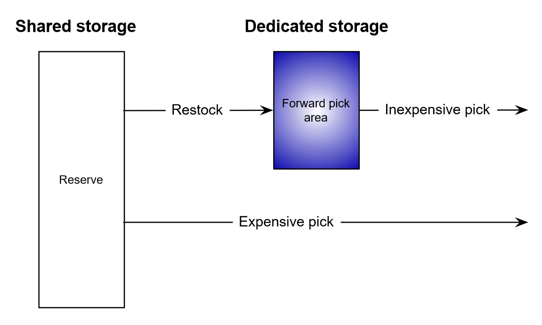
7.4 Fast-, Forward-, or Primary-Pick Area

Depending on the frequency of piecepicking, a fast-pick area may be established to optimize picking efficiency. This is a sub-region of the warehouse concentrating picks and orders within a small physical space.

The fast-pick area typically holds the most popular SKUs in small amounts, leading to less unproductive travel times and increased responsiveness to customer demand. On the other hand, large and slow-moving SKUs are better picked from the reserve area (see Figure 7.8).

As piece-picking has become more frequent, the importance of optimizing the fast-pick area has grown. This can involve adjusting the layout, storage methods, and replenishment strategies to ensure that the most frequently picked items are easily accessible.

Figure 7.8: Large/slow-moving SKUs are better picked from the reserve area (Bartholdi and Hackman 2019)

fast-pick pic: Page 133 2023-05-27#9:40 am

“Piece-picking is the most labor intensive activity in the warehouse because the product is handled at the smallest units-of-measure. Furthermore, the importance of piecepicking has greatly increased because of pressures to reduce inventory while expanding product lines. Warehouses that, 20 years ago, might have shipped cartons to customers now ship pieces and much more frequently. In a typical operation pieces are picked from cartons and neither picking nor restocking is unit-load, as shown in Figure 8.1. One of the first efficiencies a warehouse should consider is to separate the storage and the picking activities. A separate picking area, sometimes called a fast-pick or forward pick or primary pick area, is a sub-region of the warehouse in which one concentrates picks and orders within a small physical space. This can have many benefits, including reduced pick costs and increased responsiveness to customer demand. However, there is a science to configuring the fast-pick area.” (John J. Bartholdi and Steven T. Hackman, 2019, p. 99) (pdf)

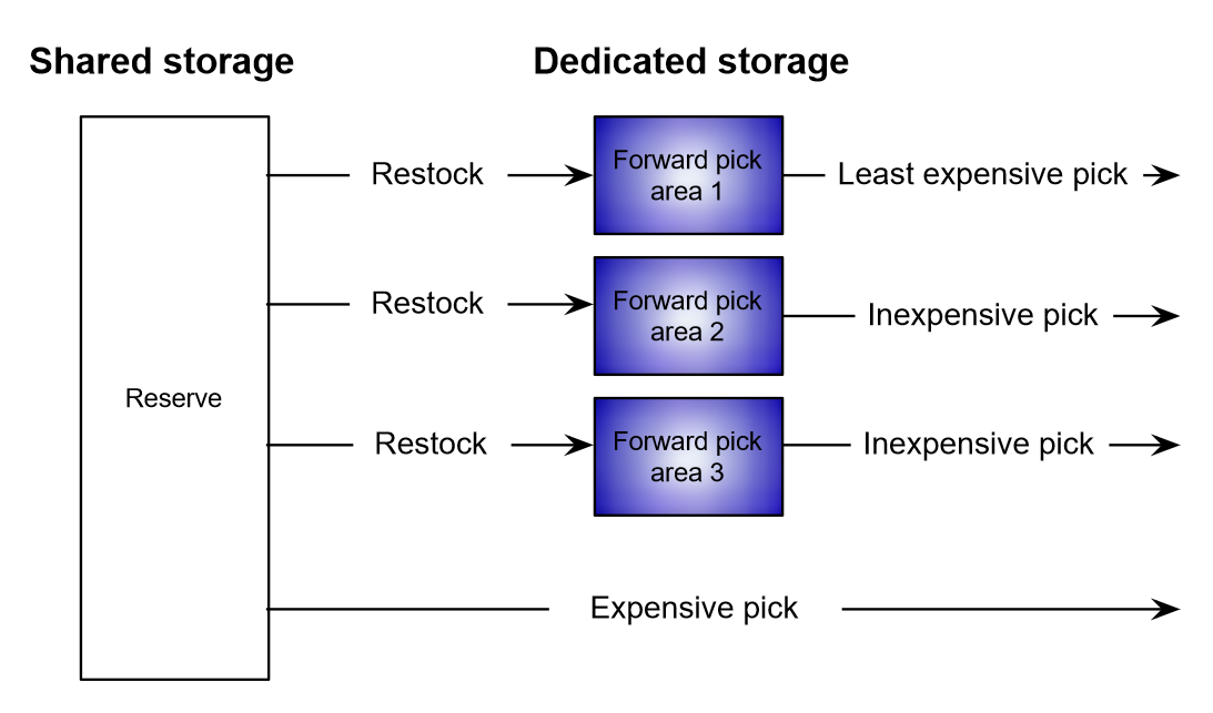
Sometimes, multiple fast-pick areas are established to further enhance picking efficiency. These areas can be strategically located based on the flow of goods and the specific picking patterns observed in the warehouse. For example, a warehouse may have separate fast-pick areas for different product categories or for different picking methods (e.g., manual picking vs. automated picking). Figure 7.9 illustrates how different picking areas may have different economics, with Forward pick area 1 leading to the least expensive picks, which may be due to its optimal location, material handling equipment, and layout design.

Figure 7.9: Pick areas may have different economics (e.g., flow-rack, carousel) (Bartholdi and Hackman 2019)

Page 143 2023-05-31#6:13 pm

---

7.4.1 Most Convenient Locations

The most convenient storage locations depend on input and output positions. Proximity to these positions is key to minimizing travel time and distance for both incoming and outgoing goods.

For example, in a flow-through layout (Figure 7.10 (a)) the best locations are near the midline between docks. Conversely, in a U-shaped layout the best locations are near the shared dock wall (Figure 7.10 (b)).

(a) Flow-through layout

(b) U-shaped layout

Figure 7.10: The most convenient storage locations are those closest to the input/output (I/O) positions, as these minimize travel time and distance. Lighter areas indicate proximity to the I/O positions.

Page 88 2023-06-01#1:03 pm

Page 88 2023-06-01#1:02 pm

7.4.2 Setting Up a Fast-Pick Area

When setting up a fast-picking area, the main questions to consider are:

• Which SKUs to store? If the SKU is high-velocity (i.e., fast-moving), it is a candidate for the fast-pick area.
• How much of each SKU to store? Overstocking an SKU can occupy valuable space that could be used for other high-velocity SKUs, while understocking can lead to frequent replenishment from reserve, which can increase costs and reduce efficiency.

It is important to strike a balance between having enough inventory on hand to meet demand and not overloading the fast-pick area with too much stock. Otherwise, the net benefits of having a fast-pick area on orderpicking may be negated by the costs of replenishment.

Trade-off: The fast-pick area may require replenishment from reserve.

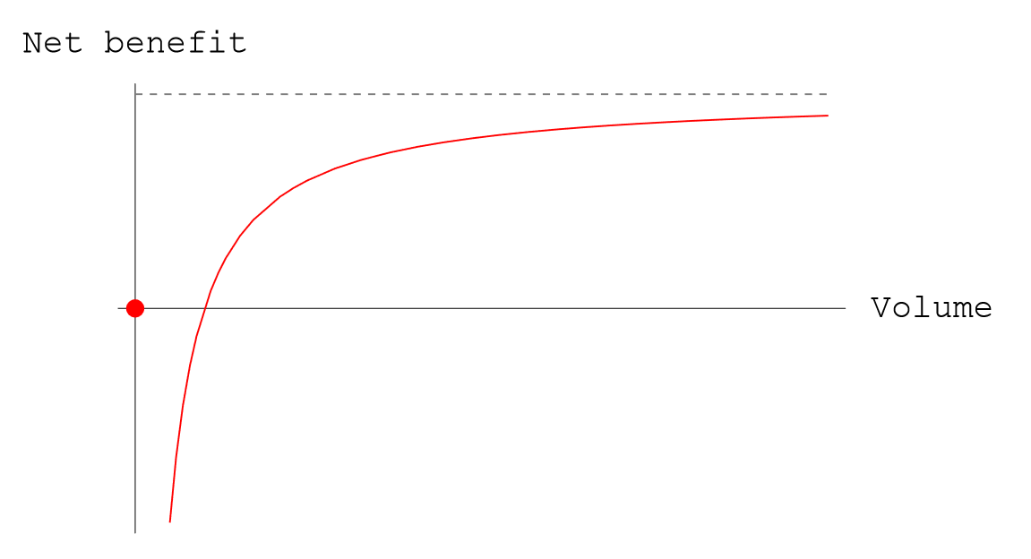
Net benefit is zero if SKU is not stored, but restock costs consume any pick savings if too little is stored.

“The fast-pick area of a warehouse functions as a “warehouse within the warehouse”: Many of the most popular stock keeping units (SKUs) are stored there in relatively small amounts, so that most picking can be accomplished within a relatively small area. This means that pickers do less unproductive travel and may be more easily supervised. The trade-off is that the fast-pick area may require replenishment from bulk storage, or reserve. The basic issues in the design of a fast-pick area are • Which SKUs to store in the fast-pick area? And • How much of each SKU to store.” (John J. Bartholdi and Steven T. Hackman, 2019, p. 99) (pdf)

Net-benefit = Page 135 2023-05-31#6:17 pm

“Congestion There are two types of congestion to which order-picking is susceptible. • Interference at a location, when both pickers want to pick from the same small area of the warehouse. • Interference in an aisle: when one worker wants to pass another but is unable to because of the narrowness of the aisle. Locations of popular SKUs are susceptible to both types of congestion because many pickers will stop there. And the congestion will be even worse if the product is requested in large quantities because order-pickers will take longer at that location.
These issues could be seen at an auto parts distributor in Indianapolis. Their philosophy was to let orders accumulate to get pick-density, and then use many pickers on a single shift. To reduce congestion in picking, they distributed the most popular product throughout the warehouse on the ground level. One problem with this approach was that it created congestion on the dock, as freight had to be staged and sorted before loading. An alternative approach would be to reduce congestion by using fewer order pickers over two shifts, which would allow concentration of popular product into fewer aisles, for less travel. The simplest model of congestion is to estimate the probability of multiple orderpickers being in the same aisle at the same time. One might do that by assuming that, for any one picker, the probability of being in an aisle is proportional to the historical number of requests from that aisle. This captures the obvious intuition that orderpickers are more likely to be in an aisle containing more popular SKUs.” (John J. Bartholdi and Steven T. Hackman, 2019, p. 88) (pdf)

7.5 Design Model for Warehouse Space Allocation

Sunderesh S. Heragu (2022) proposes a model to decide the optimal allocation of SKUs to flows. Figure 7.11 illustrates typical product flows in a warehouse. Four main flows are considered:

• (Flow 1) Receiving ➤ Cross docking ➤ Shipping: Products are passed on to customers or next facility in the supply chain.
• (Flow 2) Receiving ➤ Reserve ➤ Shipping: Products are stored in the reserve area, and order-picking operation is performed as required.
• (Flow 3) Receiving ➤ Reserve ➤ Forward ➤ Shipping: Products are
  1. stored in the reserve area (typically in pallet loads),
  2. broken into smaller loads (cartons or cases), and
  3. moved to the forward area for fast order picking.
• (Flow 4) Receiving ➤ Forward ➤ Shipping: Products are directly put into forward area to perform order consolidation (common in supplier warehouses).

Figure 7.11: Warehouse typical product flow (based on Sunderesh S. Heragu 2022)

7.5.1 Index Sets

Table 7.1: Index Sets for Optimization Model.

Symbol	Description
\(i\)	product index, \(i=1,\dots, n\)
\(j\)	flow index, \(j\in \{1,2,3,4\}\)

7.5.2 Parameters

Table 7.2 describes the parameters necessary to determine the EOQ.

Table 7.2: MIP model parameters to calculate the EOQ

Symbol	Description
\(D_{i}\)	Annual demand rate of product \(i\) in unit loads
\(C_{i}^{\mathrm{order}}\)	Order cost for product \(i\)
\(P_i\)	Price per unit load of product \(i\)
\(C^{\mathrm{carry}}\)	Carrying cost/unit of inventory/year (%) rate
\(Q_i\)	Order quantity for product \(i\) (in unit loads)
\(T_i\)	Avg. dwell time (in years) per unit load of product \(i\)

EOQ (\(Q_i^*\)). For a given product \(i\):

• order cost \(C_{i}^{\mathrm{order}}\)
• annual demand rate \(D_{i}\)
• inventory carrying cost rate/unit/year \(C_{i}^{\mathrm{carry}}\)
• price per unit load \(P_i\)
• inventory carrying cost/unit/year \(P_iC_{i}^{\mathrm{carry}}\)

The optimal order quantity is: \[ Q_i = \sqrt{\frac{2D_{i}C_{i}^{\mathrm{order}}}{P_iC^{\mathrm{carry}}}} \]

Within each replenishment cycle inventory declines linearly from \(Q_i\) to \(0\). The average on-hand over the cycle is \(Q_i/2\).

NoteExample of EOQ calculation

• \(C_{i}^{\mathrm{order}}\) = $200 per order
• \(D_{i}\) = 3,600 units/year
• \(C_{i}^{\mathrm{carry}}\) = 25%
• \(P_i\) = $100 per unit
• \(P_iC_{i}^{\mathrm{carry}} = 100 \times 25\% = \$25\)/unit/year

The optimal order quantity is:

\[ \begin{align} Q_i = & \sqrt{\frac{2 \times 3,600 \times 200}{25}} \\ = & 240 \; \text{units}\\ \end{align} \]

Average dwell time \(T_i\) (turnover time). Average duration a product stays in the shelf (time between two successive replenishments).

• Known or estimated by the warehouse manager.

• Can be estimated using the EOQ⁴ \(Q_{i}\) and annual demand \(D_{i}\) of product \(i\):

  1. The cycle time is \(\frac{Q_{i}}{D_{i}}\) years.
  2. The avg. dwell time is \(T_i = \frac{Q_i}{2D_{i}}\) years.
  3. The avg. n. of turns is \(\frac{1}{T_i} = \frac{2D_{i}}{Q_i}\).
  4. The avg. annual load is \(D_iT_i = \frac{Q_i}{2}\) units.

NoteExample of dwell time calculation

• \(Q_{i}\) = 240 units
• \(D_{i}\) = 3,600 units/year
• cycle time = \(\frac{240}{3,600} = \frac{1}{15} \; \text{years}\)
• Number of replenishments/reorders = 15

The avg. dwell time is:

\[ \begin{align} T_i = & \frac{240}{2 \times 3,600} = \frac{1}{\underbrace{30}_{\substack{avg. \\ turns}}} \; \text{years (3.2 weeks)}\\ \end{align} \]

The avg. annual load is

\[ \frac{Q_i}{2} = \frac{240}{2} = 120\; \text{units} \]

Table 7.3 describes the parameters used in the optimization model to assign SKUs to material flows and calculate costs.

Table 7.3: MIP model parameters

Symbol	Description
\(C_{ij}^{\mathrm{handle}}\)	Cost of handling a unit load of product \(i\) in material flow \(j\)
\(C_{ij}^{\mathrm{store}}\)	Cost of storing a unit load of product \(i\) in material flow \(j\) per year
\(\rho_{i}^{\mathrm{R}}\)	Average percentage of time a unit load of product \(i\) spends in the reserve area if product is assigned to material flow 3
\(d_i\)	Ratio of the size of the unit load in the reserve area to that in the forward area
\(q_{ij}\)	Break-bulk-factor5: = \(1\) if product \(i\) is assigned to material flow \(j \in \{1,2,4\}\) = \(\lceil d_i \rceil + 1\) when product \(i\) is assigned to flow \(j =3\)

Regarding costs, it is important to distinguish between:

• Inventory holding costs (\(C^{\mathrm{carry}}\)) depend only on the value of the inventory, not on its location.
• Storage costs (\(C_{ij}^{\mathrm{store}}\)) depend on the area in which the product is stored. Typically, cross-docking and forward areas carry a premium (prime real estate in a warehouse), while reserve areas tend to be cheaper.
• Storage costs (\(C_{ij}^{\mathrm{store}}\)) of product \(i\) in material flow \(j\) are typically depend on:
  • The size of a product’s unit load.
  • Warehouse leasing/construction costs per square foot.
  • Shelving type used in each area encompassing flow \(j\).
  • Accessibility and efficiency of the storage area. For example, cross-docking and forward areas may carry higher costs due to their prime location and the need for quick access whereas reserve areas may have lower costs.
• Handling costs (\(C_{ij}^{\mathrm{handle}}\)) of product \(i\) in material flow \(j\) are a function of:
  • Product size.
  • Product handling characteristics.
  • Material handling system used in the area(s) included in flow \(j\).

7.5.3 Decision Variables

Table 7.4: MIP model variables

Symbol	Description
\(x_{ij}\)	\(1\) if product \(i\) is assigned to flow type \(j\); \(0\) otherwise
\(w^{\mathrm{CD}}\)	Proportion of available space assigned to the cross-docking functional area
\(w^{\mathrm{R}}\)	Proportion of available space assigned to the reserve functional area
\(w^{\mathrm{F}}\)	Proportion of available space assigned to the forward functional area

7.5.4 Objective

Minimize total annual material handling and storage costs:

\[ \min \sum_{i=1}^{n} \sum_{j=1}^{4} t_{j} \, C^{\mathrm{handle}}_{ij} \, D_i \, q_{ij} \, x_{ij} \; + \; \sum_{i=1}^{n} \sum_{j=1}^{4} \frac{Q_i}{2} \, C^{\mathrm{store}}_{ij} \, q_{ij} \, x_{ij} \]

where \(t_{j}\) counts handling transactions for flow \(j\). Adjust \(t_j\) if operations differ:

• \(t_1=2\) for cross-docking pass (stage at cross-dock and ship),
• \(t_2=2\) for reserve only (stage at reserve and ship),
• \(t_3=3\) for reserve to forward to ship (stage at reserve, restock to forward, and ship),
• \(t_4=2\) for direct forward to ship (stage at receive and ship).

Recall that:

Handling costs

• \(2C_{ij}^{\mathrm{handle}}\) = each product \(i\) incurs 2⁶ handling transactions (receiving, shipping)
• \((2C_{ij}^{\mathrm{handle}})D_{i}\) = annual handling costs

Storage costs

• \(\frac{Q_{i}}{2}\) = avg. annual load of \(i\)
• \(\frac{Q_{i}}{2}C_{ij}^{\mathrm{store}}\) = avg. yearly storage cost of product \(i\) in material flow \(j\)

“The model also assumes that each product incurs two material-handling transactions—one for receiving and another for shipping, regardless of the area it is assigned to. If products assigned to a particular flow require more than two (or only one) material-handling transactions, the coefficient of the corresponding terms in the objective function must be appropriately weighted. For example, in some cases, the products assigned to the combined forward/reserve flow may incur three transactions, one for receiving at the reserve area, another for shipping to forward area, and a third for shipping. If this is the case, that term must have a coefficient of 3.” (Heragu, 2022, p. 289) (pdf) Handling costs

7.5.5 Constraints

• SKU-to-flow assignment: Each SKU is assigned to only one type of material flow:

  \[ \begin{align} \sum_{j}^{4}{x_{ij}} = 1 & \quad \text{for} \; i = 1,2,3, \dots, n \\ \end{align} \]

  If a single product could be allocated to multiple flows:

  • Create additional product versions with demands proportional to the different flow ratios.
  • Notice that, despite the initial estimative, the model may provide a different assignment based on the total costs.

NoteExample of SKU-to-flow assignment

Example: A manager estimates that a product has a 10,000 demand and is likely to be split on a 7:3 ratio to reserve:cross-docking. This ratio results in creating two artificial products with demands of 7,000 and 3,000.

“Constraint (2) ensures that each product is assigned to only one type of material flow. If the same product could be allocated to multiple flows due to different demand patterns, then our model requires that the manager at least knows or can estimate the percentage of this product that could be assigned to two or more of the four flows. For modelling purposes, additional versions of this product are then created (depending upon how many flows this product could be assigned to) with the demand data appropriately reduced. For example, assume that 70% of a certain product whose demand is a 10 000 units per year on average is likely to be assigned to one of the four flows, say reserve storage and another 30% to another, say cross-docking. For modelling purposes, an additional version of this product is therefore created with demand equal to 7000 and 3000 for the two products. Note that although the manager might assume that the product is likely to be split on a 7:3 ratio to reserve:cross-docking, the model may provide a different assignment based on the total costs.” (Heragu * et al., 2005, p. 333) (pdf)

• Functional area space: The SKUs assigned to each area are such that their collective space requirement is within the allotted cubic space.

  \[ \begin{align} \sum_{i=1}^{n}{\frac{Q_{i}}{2}S_{i}x_{i1}} &\leq w^{\mathrm{CD}} (z^{\mathrm{CD}}S^{\mathrm{total}}) & \text{Cross docking (flow 1)} \\ \sum_{i=1}^{n}{\frac{Q_{i}}{2}S_{i}x_{i2}} + \sum_{i=1}^{n}{\frac{Q_{i}}{2}\rho_{i}^{\mathrm{R}}S_{i}x_{i3}} &\leq w^{\mathrm{R}}(z^{\mathrm{R}} S^{\mathrm{total}}) & \text{Reserve (flows 2 and 3)}\\ \sum_{i=1}^{n}{\frac{Q_{i}}{2}(1-\rho_{i}^{\mathrm{R}})S_{i}x_{i3}} + \sum_{i=1}^{n}{\frac{Q_{i}}{2}S_{i}x_{i4}} &\leq w^{\mathrm{F}} (z^{\mathrm{F}}S^{\mathrm{total}}) & \text{Forward (flows 3 and 4)}\\ \end{align} \]

  Notice that \(\rho_{i}^{\mathrm{R}}\) is the average percentage of time a unit load of product \(i\) spends in the reserve area when assigned to flow \(3\).

• All available space is allocated: Ensures 100% of the space available is allocated to the three areas:

  \[ \begin{align} w^{\mathrm{CD}} + w^{\mathrm{R}} + w^{\mathrm{F}} = 1 \quad \end{align} \]

• Space lower and upper limits: Enforce upper and lower limits on the space that can be allocated to the cross-docking, forward, and reserve areas:

  \[ \begin{align} LL_{\mathrm{CD}}\leq w^{\mathrm{CD}} (z^{\mathrm{CD}}S^{\mathrm{total}}) \leq UL_{\mathrm{CD}}\quad \\ LL_{\mathrm{R}} \leq w^{\mathrm{R}} (z^{\mathrm{R}} S^{\mathrm{total}}) \leq UL_{\mathrm{R}}\quad \\ LL_{\mathrm{F}} \leq w^{\mathrm{F}} (z^{\mathrm{F}} S^{\mathrm{total}}) \leq UL_{\mathrm{F}}\quad \end{align} \]

“Constraints (8.8) through (8.10) serve to enforce upper and lower limits on the space that can be allocated to the cross-docking, forward, and reserve areas.” (Heragu, 2022, p. 290) (pdf)

• Non-negativity: Ensure that the decision variables are non-negative and available space proportions are within the range \([0,1]\):

  \[ \begin{align} x_{ij} \in \{0,1\} & \quad \text{for all products} \; i \; \text{and flows} \; j\\ w^{\mathrm{CD}}, w^{\mathrm{R}}, w^{\mathrm{F}} \geq 0 & \quad \text{(proportion of available spaces)} \end{align} \]

Example

“Example 8.2 A warehouse handles six classes of products. The average annual demand, order cost, price, and space required per unit load for each class of product is shown in Table 8.1. Assuming a carrying cost rate of 10%, total available space of 100,000 square meters, determine how the products should be allocated to each of the four areas. Assume the handling and storage costs given in Table 8.2, an upper and lower bound of 75,000 and 35,000 square meters for reserve and forward areas and a maximum of 15,000 square meters for the cross-docking area. Also, assume a = b = c = 1, pi = 0.2 and 1 for products 3 and 6, 0 for all others, and qi3 = 1 for i = 1, 2, …, 6.” (Heragu, 2022, p. 290) (pdf)

Here’s the heuristic algorithm reformatted with each step on a new line and content using inline LaTeX:

• Step 1: For each \(i = 1, 2, \dots, n\), find \(\min_{j=1, 2, 3, 4} \left( 2q_{ij}H_{ij}\lambda_i + q_{ij}C_{ij}Q_i/2 \right)\). Let \(j = j^*\), where the minimum occurs. Set \(X_{ij^*} = 1\) and \(X_{ik} = 0\) for \(k = 1, 2, 3, 4, k \neq j^*\).
• Step 2: Calculate \(\alpha\), \(\beta\), and \(\gamma\) using equations (16–18). If \(\alpha + \beta + \gamma > 1\), stop because the problem is infeasible. Otherwise, go to Step 3.
• Step 3: Calculate the upper bounds \(\alpha_{UB} = \frac{UL_{CD}}{aTS}\), \(\beta_{UB} = \frac{UL_R}{bTS}\), and \(\gamma_{UB} = \frac{UL_F}{cTS}\). If \(\alpha \leq \alpha_{UB}, \beta \leq \beta_{UB}, \gamma \leq \gamma_{UB}\), stop because there is a feasible, optimal solution. Otherwise, go to Step 4.
• Step 4: Let \(\max \left\{ \alpha - \alpha_{UB}, \beta - \beta_{UB}, \gamma - \gamma_{UB} \right\}\) occur for area \(k, k = 1, 2, 3\), and \(\min \left\{ \alpha - \alpha_{UB}, \beta - \beta_{UB}, \gamma - \gamma_{UB} \right\}\) occur for area \(l, l = 1, 2, 3\). Set \(k^* = k\) and \(l^* = l\). Place \(k^*\) in set \(P\), \(l^*\) in set \(Q\), and the remaining index \(m\) in \(P\) if the total space coefficient exceeds the upper bound; otherwise, place \(m\) in \(Q\).
• Step 5: Pick a product \(i^*\) in area \(k^*\) and move it to area \(l^*\), provided:
  1. the upper bound space constraint in \(l^*\) is not violated, and
     
  2. \(\left( 2q_{li^*}H_{li^*}\lambda_{i^*} + q_{li^*}C_{li^*}Q_{i^*}/2 \right) - \left( 2q_{ik^*}H_{ik^*}\lambda_{i^*} + q_{ik^*}C_{ik^*}Q_{i^*}/2 \right)\) is minimized for \(i = i^*\).
     If no product satisfies these conditions, set \(k^* = m\) and repeat Step 5. If no feasible reassignment exists, stop.
• Step 6: If the current solution is feasible, stop. Otherwise, return to Step 2.

\(\alpha = \sum_{i=1}^n \left( Q_i S_i X_{i1} / 2 \right) / a TS\) \(\beta = \sum_{i=1}^n \left( Q_i S_i X_{i2} / 2 \right) + \sum_{i=1}^n \left( p_i Q_i S_i X_{i3} \right) / b TS\) \(\gamma = \sum_{i=1}^n \left( (1 - p_i) Q_i S_i X_{i3} / 2 \right) + \sum_{i=1}^n \left( Q_i S_i X_{i4} / 2 \right) / c TS\)

These equations define the relationships between variables related to product allocation and warehouse design.

7.6 Worked Example

We illustrate parameterization and a baseline allocation with 6 SKUs. Carrying rate is \(C^{carry}=0.10\). Total space is \(S^{total}=100,000\) \(m^2\). Bounds: reserve and forward each between \(35,000\) and \(75,000\), cross-docking at most \(15,000\).

Table 7.5: SKU Data for Worked Example.

SKU	\(D_i\)	\(C_i^{order}\)	\(P_i\)	\(S_i\) \((m^2)\)
1	2500	120	60	2.0
2	1500	160	40	1.5
3	900	250	90	3.0
4	3200	180	30	1.2
5	600	140	70	2.2
6	1100	200	50	1.8

Compute EOQ and average annual load.

\[ Q_i = \left( \frac{2 D_i C_i^{order}}{P_i C^{carry}} \right)^{1/2}, \quad \text{average annual load is } Q_i/2. \]

import math, pandas as pd
rows=[
    {"SKU":1,"D":2500,"Co":120,"P":60,"S":2.0},
    {"SKU":2,"D":1500,"Co":160,"P":40,"S":1.5},
    {"SKU":3,"D":900,"Co":250,"P":90,"S":3.0},
    {"SKU":4,"D":3200,"Co":180,"P":30,"S":1.2},
    {"SKU":5,"D":600,"Co":140,"P":70,"S":2.2},
    {"SKU":6,"D":1100,"Co":200,"P":50,"S":1.8},
]
carry=0.10
df=pd.DataFrame(rows)
df["Q"] = ((2*df.D*df.Co)/(df.P*carry))**0.5
df["Q/2"] = df["Q"]/2
df_round=df[["SKU","D","Co","P","S","Q","Q/2"]].round(1)
df_round

	SKU	D	Co	P	S	Q	Q/2
0	1	2500	120	60	2.0	316.2	158.1
1	2	1500	160	40	1.5	346.4	173.2
2	3	900	250	90	3.0	223.6	111.8
3	4	3200	180	30	1.2	619.7	309.8
4	5	600	140	70	2.2	154.9	77.5
5	6	1100	200	50	1.8	296.6	148.3

Handling multipliers. Use \((t_1,t_2,t_3,t_4)=(2,2,3,2)\) to reflect an extra transfer when moving from reserve to forward before shipping.

Cost matrices. Calibrate to your equipment and wages. A teaching set is below in money per unit-load and per unit-load-year.

Flow \(j\)	\(C^{handle}\)	Rationale
1 cross-dock	3.0	receive and ship pass with sorting
2 reserve	5.0	longer travel and putaway or retrieval
3 reserve+forward	7.0	receive, transfer, ship
4 forward	4.0	short travel inside forward area

Area	\(C^{store}\)	Rationale
Cross-dock	1.5	premium floor near dock
Reserve	0.8	high-density storage
Forward	2.0	prime picking real estate

Set \(q_{ij}=1\) except use \(q_{i3} = \lceil d_i \rceil + 1\) if breaking pallets into cases in flow 3. If detailed pack ratios are unknown set \(q_{i3}=1\) for a first pass.

Baseline allocation. For each SKU compute four objective coefficients \[ K_{ij} = t_j C^{handle}_{ij} D_i q_{ij} + (Q_i/2) C^{store}_{ij} q_{ij}. \]

Choose the smallest \(K_{ij}\), then adjust to satisfy area bounds by moving the least costly marginal SKUs. This greedy baseline provides a feasible solution that the MIP can improve.

Space checks. Compute left-hand sides of the capacity constraints using \(Q_i/2\) and \(S_i\) with the chosen flows, then scale by vertical levels. If bounds fail, reassign the smallest-cost-delta SKU from the tight area to an underfilled area.

Managerial note. If \(C^{store}_{forward}\) is high but \(C^{handle}_{forward}\) is low, only high-demand SKUs with small \(S_i\) should enter the forward area.

7.7 Sensitivity Analysis

• Area bounds: tightening \(UL_F\) often shifts marginal SKUs from forward to reserve and increases handling costs due to added travel.
  
• Carrying rate: increases in \(C^{carry}\) reduce \(Q_i\) and lower average annual load, easing space pressure.
  
• Handling multipliers: if reserve to forward transfers are mechanized, reduce \(t_3\) and more SKUs may justify the forward path.
  
• Lane depth: increasing depth at fixed aisle width raises total pallet positions but can degrade FIFO and flexibility. Evaluate honeycombing exposure before changing depth.

7.8 Implementation Guidance

1. Collect demand and price data from ERP to compute \(Q_i\) and \(Q_i/2\).
   
2. Map existing equipment and aisle widths to estimate area-specific storage costs.
   
3. Use time studies or engineered standards to estimate handling costs per flow.
   
4. Calibrate \(q_{ij}\) for break-bulk effects in flow 3.
   
5. Solve the MIP and validate against floor constraints and safety stock policies.
   
6. Pilot a forward-area set with congestion monitoring before full rollout.

7.9 Limitations and Extensions

• The model is single period. Seasonality can be handled by a multi-period extension with time-indexed capacities.
  
• Congestion is not modeled explicitly. A post-processing rule can limit pick density per aisle.
  
• Stochastic demand and service-level constraints can be integrated via safety stock that inflates \(Q_i/2\) or via chance constraints.
  
• If multiple pack sizes exist per SKU, treat each pack as a product with its own demand and size.

7.10 Summary

• Model simultaneously considers the product allocation and functional area sizing problems in the design of a warehouse.
• Solve the two problems jointly to minimize annual handling and storage costs.
• Input data requirements readily available in most warehouses.
• Model can be solved to optimality on 3,000 SKUs using commercial MILP solvers.
• For larger problems (e.g., 150,000 SKUs), see (meta-)heuristic solutions in (S. S. Heragu et al. 2005).
• For a multi-step approach including decisions on functional areas, travel distances, and storage strategies (e.g., dedicated, class-based, randomized) (see Huuskes 2023).

“This paper has simultaneously considered the product allocation and functional area size determination problems in the design of a warehouse. It provides a mathematical model and a heuristic algorithm to solve the two problems jointly so that annual handing and storage costs can be minimized. The input data requirement for this model is readily available in most warehouses and the model considers realistic constraints. We believe this is the only available model that considers the two problems simultaneously and allows the user to solve them optimally.” (Heragu et al., 2005, p. 337) (pdf)

7.11 Exercises

7.11.1 Exercise 1. Space utilization in a warehouse lane

Consider the pallet positions A, B, C, shown in Figure 7.12. If the warehouse has a single SKU occupying these positions and the demand is 1 pallet per day. Each pallet position occupies area \(p\) and the aisle space in front of the pallet is of area \(a/2\).

• What is the utilization rate \(u_{A}\), \(u_{B}\), and \(u_{C}\) for each position?
• What is the total unoccupied area across the three days for the lane in terms of \(p\) and \(a\)?

Figure 7.12: Pallet positions A, B, and C with area \(p\) and aisle front area \(a/2\). SKU demand is 1 pallet per day.

TipAnswer

We analyze the occupancy of each pallet position over three days, given that one pallet is removed each day from the front position (i.e., position C). The utilization rate for each position is:

• \(u_{A} = 1\)
• \(u_{B} = 2/3\)
• \(u_{C} = 1/3\)

The total unoccupied area-days for the lane is calculated as follows:

• Day 1: \(\frac{a}{2}\)
• Day 2: \(p + \frac{a}{2}\)
• Day 3: \(2p + \frac{a}{2}\)

Total: \(3p + \frac{3a}{2}\)

7.11.2 Exercise 2. Functional Areas and Functions

Match each function with an area:

• Receiving
• Shipping
• Staging for Cross-Docking
• Reserve
• Forward Pick

#	Function	Functional Area
1	Optimized for order collation and rapid replenishment.
2	Pallet loads or individual cartons of products are received.
3	Picked order items are staged and value-added services are performed.
4	In cross-docking, products are sorted for outbound operations.
5	Performs value-added operations such as labeling or kitting.
6	Received products are pre-sorted.
7	Products are staged briefly then moved to shipping or storage.
8	High-density storage equipment is used to maximize space utilization.
9	Smaller storage area designed for fast order picking.
10	Items wait temporarily before being moved to shipping.
11	Stores bulky products for extended periods.

TipSolution

1. Forward Pick
2. Receiving
3. Shipping
4. Staging
5. Forward Pick
6. Staging
7. Receiving
8. Reserve
9. Forward Pick
10. Staging
11. Reserve

7.11.3 Exercise 3. One Product Using Multiple Flows

Consider that a product \(p\) has a 10,000 demand and is likely to be split on a 7:3 ratio to reserve:cross-docking. However the variable \(x_{ij}\), where \(i\) is the product and \(j\) is the flow, is binary and can only be assigned to a single flow:

\[ \sum_{j}^{4} x_{ij} = 1 \quad \forall \quad i = 1, 2, 3, \ldots, n \]

How can we adjust the model to deal with this specific situation?

TipSolution

To adjust the model to deal with this specific situation, we can create additional product versions with demands proportional to the different flow ratios. In this case, we replace product \(p\) by two new articial products \(p_{1}\) and \(p_{2}\) with demands of 7,000 and 3,000, respectively. This way, each product version can be assigned to a single flow, and the model can provide the optimal assignment based on the total costs.

7.12 Review Questions

1. Define honeycombing and describe its effect on space reuse.
   
2. Explain why deeper lanes both add pallet positions and reduce flexibility.
   
3. Show how \(Q_i/2\) enters both space and storage cost terms.
   
4. When does flow 3 with reserve plus forward beat flow 2 or 4 in total cost.
   
5. List three data items needed to calibrate \(C^{handle}\) and two needed for \(C^{store}\).

7.13 Summary

We jointly allocate SKUs to flows and size functional areas using cost terms derived from handling and storage. EOQ links demand, ordering, and carrying cost to dwell time and average annual load, which drive space terms. Lane depth and forward-area configuration create important trade-offs that should be validated with sensitivity and pilot tests.

References

Accorsi, Riccardo, Giulia Baruffaldi, and Riccardo Manzini. 2017. “Design and Manage Deep Lane Storage System Layout. An Iterative Decision-Support Model.” The International Journal of Advanced Manufacturing Technology 92 (1): 57–67. https://doi.org/10.1007/s00170-016-9962-9.

Bartholdi, John J., and Steven T. Hackman. 2019. Warehouse
& Distribution Science. Release 0.98.1. The Supply Chain
& Logistics Institute, Georgia Tech. https://doi.org/10.13140/RG.2.1.4264.0481.

Derhami, Shahab, Jeffrey S. Smith, and Kevin R. Gue. 2017. “Optimising Space Utilisation in Block Stacking Warehouses.” International Journal of Production Research 55 (21): 6436–52. https://doi.org/10.1080/00207543.2016.1154216.

———. 2019. “Space-Efficient Layouts for Block Stacking Warehouses.” IISE Transactions 51 (9): 957–71. https://doi.org/10.1080/24725854.2018.1539280.

Heragu, S. S., L. Du, R. J. Mantel, and P. C. Schuur. 2005. “Mathematical Model for Warehouse Design and Product Allocation.” International Journal of Production Research 43 (2): 327–38. https://doi.org/10.1080/00207540412331285841.

Heragu, Sunderesh S. 2022. Facilities Design. Fifth edition. Boca Raton, FL: CRC Press.

Huuskes, S. 2023. “An Iterative Approach to Warehouse Tactical Level Decision Making.” BSc thesis, Enschede, The Netherlands: University of Twente, Industrial Engineering; Management. https://purl.utwente.nl/essays/94897.

Kind, D. A. 1975. “Elements of Space Utilization.” Transportation and Distribution Management 15: 29–34.

Matson, Jan O. 1982. “The Analysis of Selected Unit Load Storage Systems.” PhD thesis, Atlanta, GA: Georgia Institute of Technology.

---

1. Pallet position: Floor space for a pallet, including footprint and gaps.

2. Unit area: Warehouse expenses (e.g., rent, climate control) are typically measured per square meter.

3. Honeycombing: Unoccupied interior lane spaces unavailable for other SKUs after a retrieval.

4. EOQ (Economic Order Quantity) is the optimal order quantity that minimizes the total inventory costs, which include ordering costs and carrying costs.

5. The break-bulk-factor \(q_{ij}\) can be greater than 1 in flow 3 since \(q_{ij} = \lceil d_i \rceil + 1\) thus modifying handling and storage costs. For example, \(d_i = \frac{\text{size pallet}}{\text{size carton}} \geq 1\).

6. The model assumes that each product incurs 2 material-handling transactions but in some cases, products assigned to the combined forward/reserve flow may incur 3 transactions (receiving at the reserve area, shipping to forward area, third for shipping). So, adjust the coefficient accordingly.