10 Warehouse Storage Optimization

10.1 🎯 Aims

This assignment aims to introduce the concepts of warehouse storage optimization through mathematical modeling and analysis.

10.2 🧠 Learning Objectives

After completing this assignment, students will be able to:

Develop a mathematical optimization model for the classical storage location assignment problem (SLAP).
Compare space utilization between dedicated and randomized storage policies.

10.3 🔧 Steps

10.3.1 Summary of Tasks

Storage Location Assignment
- Distance Matrix and Weights (20%)
- Mathematical Model (SLAP) (50%)
Random vs. Dedicated Policies (30%)

10.3.2 Submission

Please follow this template to structure your answer document.

Upon finishing, submit on Canvas:

The .ipynb file with your answers.
A PDF export of your .ipynb file.

10.3.3 Assessment Criteria

Storage Location Assignment
- Distance Matrix and Weights correctly computed
- Mathematical Model correctly formulated and solved
Random vs. Dedicated Policies
- Correct computation of required storage capacities for both policies
- Clear comparison and analysis of the two policies

Evaluation Rules

Repair assignments are capped at a maximum grade of 5.5.
Students may appeal grading decisions. Appeals must reference specific rubric criteria and provide a clear justification. Appeals must be submitted within 3 days of receiving the grade.

Table 10.1: Rubric for evaluating the warehouse storage optimization assignment. Each criterion is scored from 1 to 3, with detailed descriptions for each level of performance. The total points column indicates the maximum points available for each criterion.

Label	Criterion	3 – Very Good	2 – Satisfactory	1 – Needs Improvement	Points
SLAP1	Distance Matrix	Distance measure matches grid stepping; full IO→location table correct.	Mostly correct with a few cells wrong.	Many wrong cells or inconsistent distance logic.	1
SLAP2	Weights Table	Combines IO costs, frequencies, and distances as specified; normalized per item; table correct for A, B, C, D.	Logic correct but a few entries off; item totals still usable.	Missing elements (e.g., not combining across IOs or no normalization); several wrong columns.	1
SLAP3	Objective Value	Objective value matches recomputation using submitted data and weights.	Minor mismatch due to rounding or small errors in copying values.	Significant mismatch or built from incorrect or altered inputs.	1
SLAP4	Mathematical Model	Mathematical model correct and usable.	Mathematical model mostly correct but with minor gaps.	Model is mostly incorrect (objective function or constraints missing, solver problems).	2
SLAP5	Assignment	Location numbering, rows/columns, and IO orientation are correct and consistent with the given layout.	Minor orientation slip that doesn’t change the allocation logic.	Mirrored/shifted layout leading to incorrect distances or placement.	2
POL1	Safety Stock & Period Requirements	Next-period shift correct (last period uses zero); safety stock is ten percent of next period and rounded up (ceiling); per-period required spaces correct for all items/periods.	One aspect slightly off (e.g., rounding or last period) but mostly correct.	Misapplied rule (e.g., current period used; no rounding); several periods wrong.	1
POL2	Dedicated Capacity	Per-item peaks across periods summed for total dedicated capacity.	Total slightly off.	Wrong computation logic.	1
POL3	Random Capacity	Maximum sum across periods for total random capacity.	Max slightly off.	Wrong computation logic.	1

10.4 Tasks

10.4.1 Storage Location Assignment

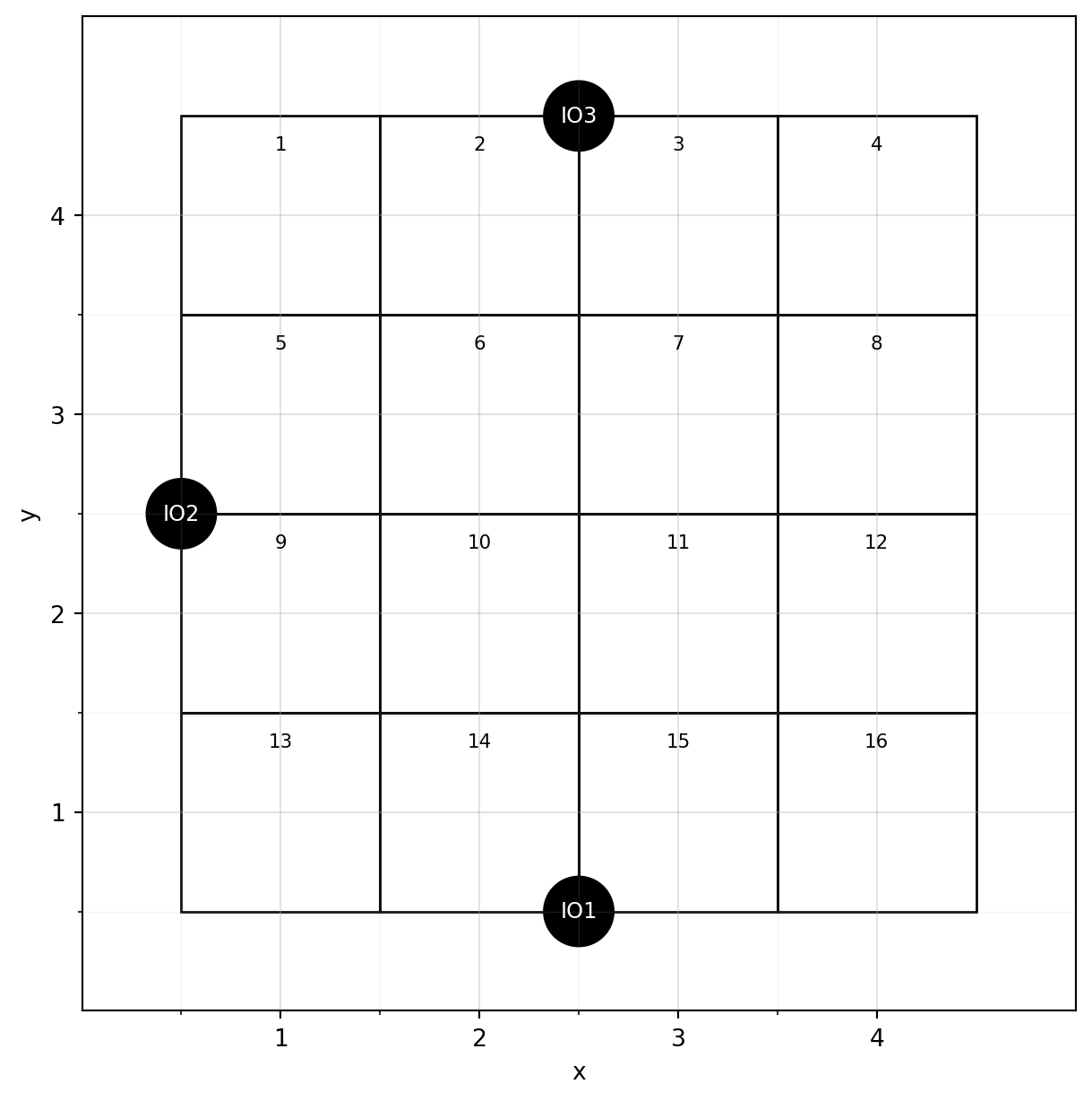
Consider the warehouse layout shown in Figure 10.1. There are three I/O points through which four items enter and leave the warehouse. All three I/O points are located on the periphery of the building, with the first equidistant from storage spaces 14 and 15, second from 5 and 9, and the third from storage spaces 2 and 3.

Figure 10.1: Warehouse layout with three I/O points and 16 same-sized storage locations.

The number of storage spaces \(S_i\) required for each of the four items is given by Table 10.2.

Table 10.2: Number of storage spaces \(S_{i}\) required for each item \(i\) totaling 16 spaces.

Item	N. of Storage Spaces
A	3
B	5
C	2
D	6

And the frequency \(f_{ik}\) of trips \(i\) for each item-I/O point \(k\) combination and cost \(c_{ik}\) of moving a unit load of item \(i\) to/from I/O point \(k\) are given in tables Table 10.3 and Table 10.4, respectively.

Table 10.3: Frequency of trips \(f_{ik}\) for each item-I/O pointcombination.

IO Point	1	2	3
Item
A	150	25	88
B	60	200	150
C	96	15	85
D	175	135	90

Table 10.4: Cost \(c_{ik}\) of moving a unit load of item \(i\) to/from I/O point \(k\).

IO Point	1	2	3
Item
A	6	5	5
B	7	3	6
C	4	7	9
D	15	8	12

We assume that the costs are influenced by the handling requirements of each item. These requirements may include factors such as weight, volume, and fragility, which can affect the type of equipment needed or the labor intensity involved.

Distance Matrix and Weights

To calculate the distance matrix and weights, follow these steps:

Distance Matrix: Compute the Manhattan distances \(d_{kj}\) between each I/O point \(k\) and storage location \(j\). The storage locations are arranged in a 2D grid, and their coordinates correspond to their centroids. For example:
- Storage location 1 is at \((1, 4)\).
- I/O point IO1 is at \((2.5, 0.5)\).
Use the formula for Manhattan distance: \[ d_{kj} = |x_k - x_j| + |y_k - y_j| \] where \((x_k, y_k)\) and \((x_j, y_j)\) are the coordinates of the I/O point and storage location, respectively.
Weights Calculation: Using the distance matrix, calculate the weights \(w_{ij}\) for each item \(i\) and storage location \(j\): \[ w_{ij} = \frac{\sum_{k=1}^{3} c_{ik} f_{ik} d_{kj}}{S_i} \] Here:
- \(c_{ik}\) is the cost of moving a unit load of item \(i\) to/from I/O point \(k\).
- \(f_{ik}\) is the frequency of trips for item \(i\) to/from I/O point \(k\).
- \(d_{kj}\) is the distance between I/O point \(k\) and storage location \(j\).
- \(S_i\) is the total number of storage spaces required for item \(i\).
Present Results: Populate the distance matrix and weights tables using the templates provided in Table 10.5 and Table 10.6. Ensure all calculations are accurate and clearly formatted for easy interpretation.

Distance Matrix and Travel Time Models

For simplicity, we assume no batching occurs during the picking process. Therefore, the travel time is directly proportional to the distance between I/O points and storage locations.

If batching were considered, the travel time would depend on the sequence and combination of storage locations visited during a single picking route. This would require a more complex travel time model, such as those used in routing problems, to account for the additional travel time incurred when picking items from multiple storage locations.

Table 10.5: Distance matrix between I/O points 1, 2, and 3 and storage locations 1–16.

IO Point	1	2	3
Location(k)
1
2
3
4
5
6
7
8
9
10
11
12
13
14
15
16

Table 10.6: Weights corresponding to the relative importance of each storage location for each item, taking into account the frequency of trips and the cost of movement.

Item(j)	A	B	C	D
Location(i)
1
2
3
4
5
6
7
8
9
10
11
12
13
14
15
16

Mathematical Model

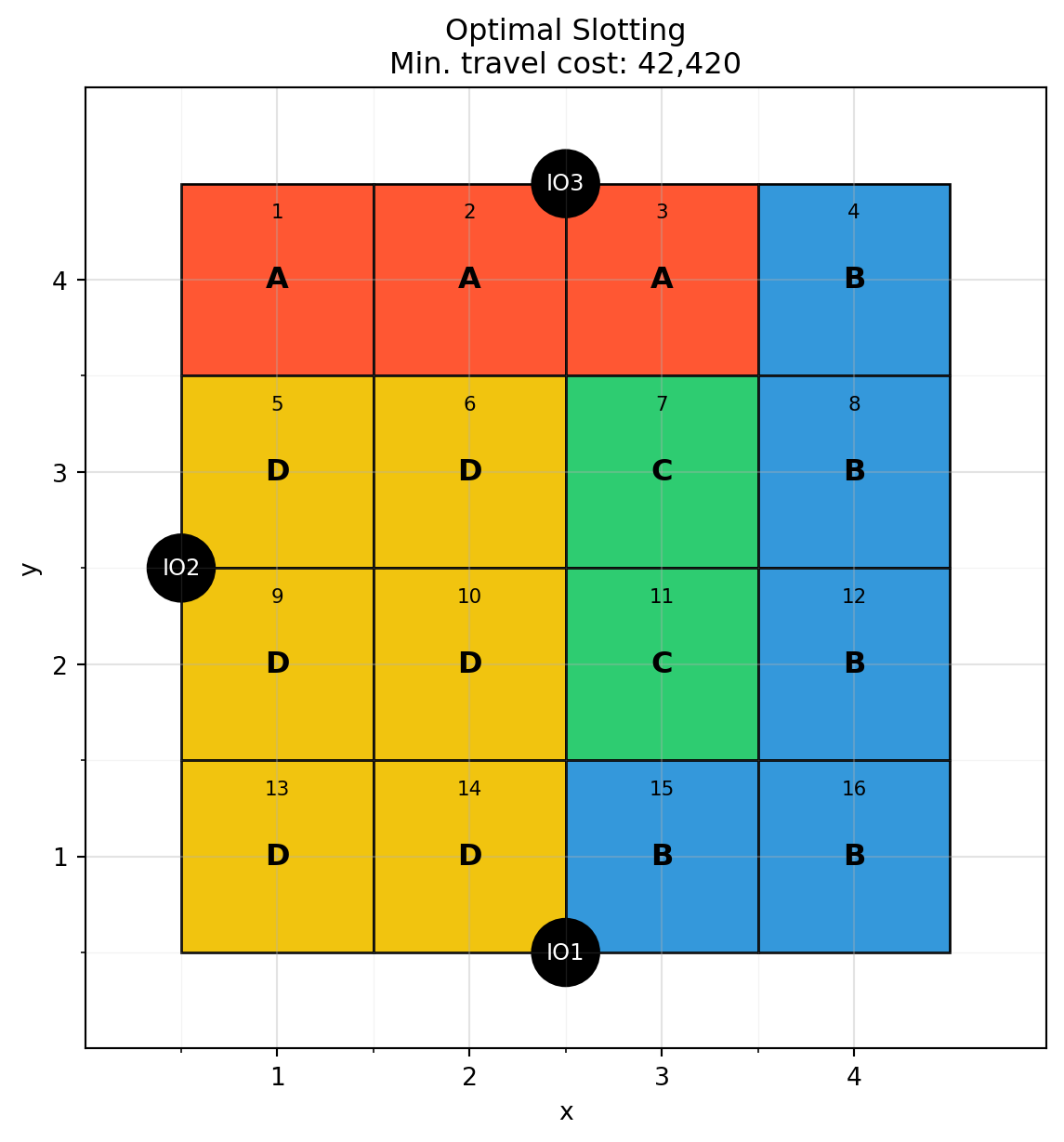
Determine the optimal allocation of the four items to the 16 storage spaces such that the total travel cost between the I/O points and the storage spaces is minimized. Provide the value of the objective function and a graphical representation of your optimal product-location assignment. An example of the expected output is shown in Figure 10.2.

Figure 10.2: Example of optimal product-location assignment (Cost = 42,420).

10.4.2 Space Allocation: Random vs. Dedicated Policies

A unit-load warehouse specializing in five high-turnover consumer items is scheduled to receive the quantities shown in Table 10.7 for the next 12 periods.

Table 10.7: Scheduled receipts for five items (A, B, C, D, and E) throughout the 12 periods.

	A	B	C	D	E
Period
1	20	12	66	22	97
2	15	8	15	22	12
3	30	4	16	25	88
4	12	6	17	21	66
5	14	7	18	18	79
6	60	1	19	14	55
7	17	12	15	23	9
8	20	40	16	36	25
9	21	13	17	30	96
10	22	12	18	22	90
11	23	12	19	89	90
12	23	12	15	22	88

The warehouse manager likes to maintain a quantity of safety stock for each product in each period equal to 10% of the scheduled receipt of that product for the next period. Determine the total storage spaces required under the dedicated and random storage policies considering the following assumptions:

Blockage is allowed (i.e., products can be stored in front of each other).
The products have same dimensions and handling requirements.
Inventory is not carried over between periods.
Safety stock is calculated as a fixed percentage (viz., 10%) of the next period’s receipt (rounded up).