Practice Exercises - Supplier Selection and Multi-Objective Optimization

Question 1

Weighted Scoring Method. Assume that all weights are 1 similar. Given the objectives provided below, provide the objective function for:

1. Maximization:

   \[ \begin{align*} \min & +2x_1 + 3x_2 - x_3 \\ \max & +4x_1 - 2x_2 \\ \max & +x_2 - x_3 \end{align*} \]

2. Minimization:

   \[ \begin{align*} \min & +3x_1 - 1 x_2 \\ \max & +4x_1 - 2x_2 + 9x_3\\ \end{align*} \]

Question 1 - Answer

Given that all weights \(w\) are assumed to be equal we have:

1. Maximization. Sum the maximization objectives and subtract the minimization objectives:

   \[ \begin{align*} \max Z = & \quad -(2x_1 + 3x_2 - x_3) + (4x_1 - 2x_2) + (x_2 - x_3) \\ = & \quad -2x_1 - 3x_2 + x_3 + 4x_1 - 2x_2 + x_2 - x_3 \\ = & \quad (4x_1 - 2x_1) + (-3x_2 - 2x_2 + x_2) + (x_3 - x_3) \\ = & \quad 2x_1 - 4x_2 \\ \end{align*} \]

2. Minimization. Sum the minimization objective and subtract the maximization objectives:

   \[ \begin{align*} \min Z = & \quad (+3x_1 - x_2) - (4x_1 - 2x_2 + 9x_3) \\ = & \quad 3x_1 - x_2 - 4x_1 + 2x_2 - 9x_3 \\ = & \quad (3x_1 - 4x_1) + (2x_2 - x_2) - 9x_3 \\ = & \quad -x_1 + x_2 - 9x_3 \\ \end{align*} \]

Question 2

Lexicographical Method. Provide the optimal solution for the lexicographic problem. Considering the first objective as the most important.

\[ \begin{align*} \max & \quad x_1 \\ \max & \quad 2x_1 + 3x_2 \\ \text{s.t.} & \quad x_1 \leq 3 \\ & \quad x_1 + x_2 \leq 5 \\ & \quad x_1, x_2 \geq 0 \end{align*} \]

Question 2 - Answer

The Lexicographical Method is a multi-objective optimization technique where objectives are ranked according to their importance, and the optimization is carried out in that order. In the given problem, the most important objective is maximizing \(x_1\), and the second priority is maximizing \(2x_1 + 3x_2\). The process can be broken down into two stages:

1. First Optimization (Objective \(f_1\))

   Here, the goal is to maximize \(x_1\) subject to the given constraints. The problem formulation is:

   \[ \begin{align*} \max & \quad x_1 \\ \text{s.t.} & \quad x_1 \leq 3 \\ & \quad x_1 + x_2 \leq 5 \\ & \quad x_1, x_2 \geq 0 \end{align*} \]

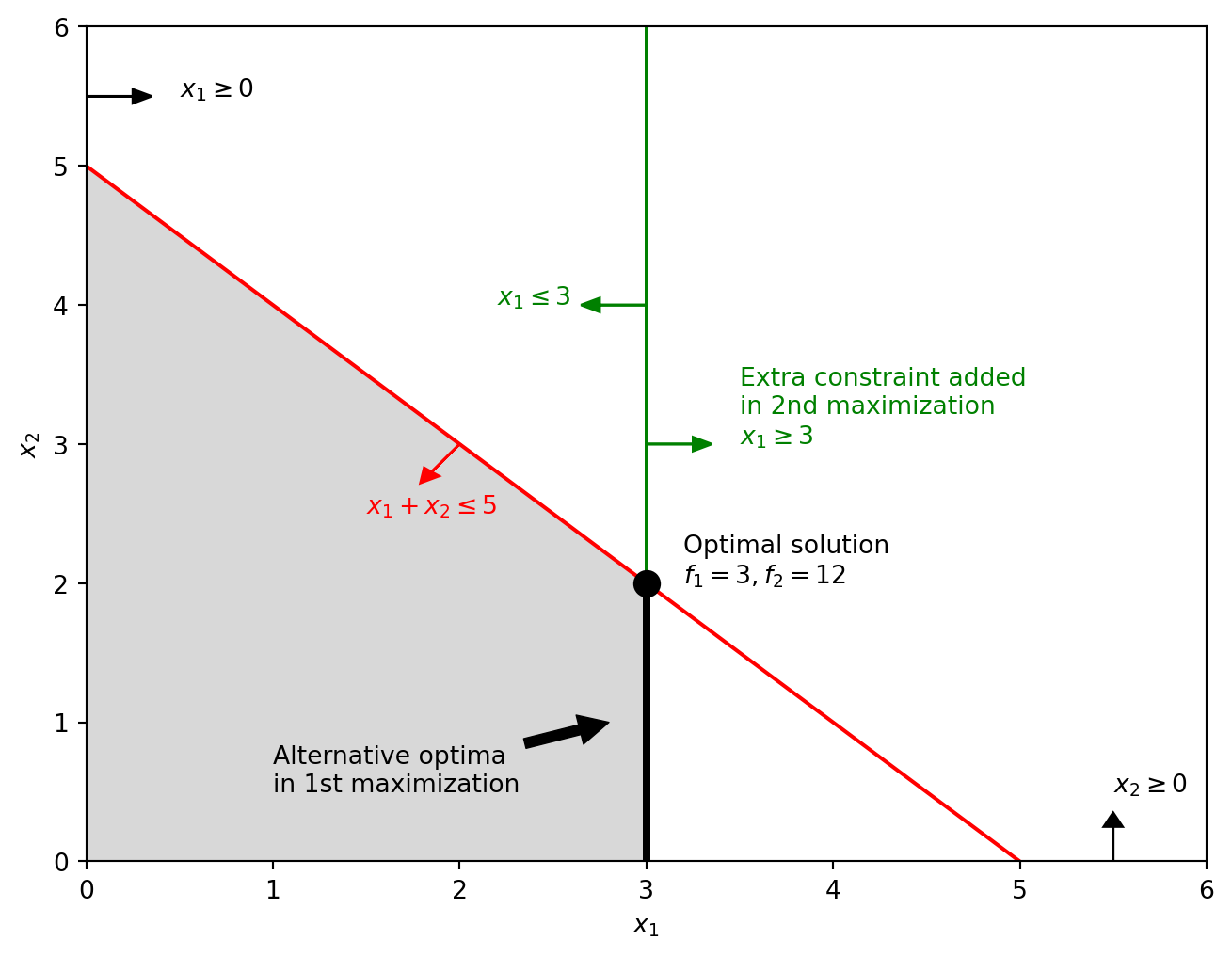
   In this stage, the focus is solely on maximizing \(x_1\) without considering \(2x_1 + 3x_2\). The optimal solution to this problem, \(x_1^*\), is determined by the most restrictive constraint on \(x_1\), which is \(x_1 \leq 3\). Therefore, the optimal value is \(x_1^* = 3\) and the corresponding objective value is \(f_1^* = 3\).

2. Second Optimization (Objective \(f_2\))

   After determining \(x_1^*\), the next step is to maximize \(2x_1 + 3x_2\) while ensuring that the primary objective value does not decrease. This leads to the introduction of an additional constraint: \(x_1 \geq x_1^*\). The new problem formulation becomes:

   \[ \begin{align*} \max & \quad 2x_1 + 3x_2 \\ \text{s.t.} & \quad x_1 \leq 3 \\ & \quad x_1 + x_2 \leq 5 \\ & \quad x_1 \geq 3 \quad \text{(Extra constraint ensuring } f_1 \geq f_1^*\text{)} \\ & \quad x_1, x_2 \geq 0 \end{align*} \]

   With \(x_1 = 3\) fixed from the first optimization, the problem reduces to:

   \[ \begin{align*} \max & \quad 6 + 3x_2 \\ \text{s.t.} & \quad 3 + x_2 \leq 5 \\ & \quad x_2 \geq 0 \end{align*} \]

   The maximum value of \(x_2\) that satisfies these constraints is \(x_2 = 2\), resulting in a secondary objective value of \(f_2 = 12\).

The final optimal solution for this lexicographic optimization problem is \(x_1 = 3\) and \(x_2 = 2\), with the primary and secondary objective values being \(f_1^* = 3\) and \(f_2^* = 12\), respectively.

Figure 1: Optimal solution for lexicographic optimization.

This approach ensures that the most important objective is optimized first, and then the next important objective is considered without compromising the already optimized higher-priority objectives.

Question 3

Goal Programming vs. Pareto Efficiency. Consider the following mathematical optimization problem:

\[ \begin{align*} \min &\quad x_1 \\ \max & \quad x_2 \\ \text{s.t.} & \quad 0 \leq x_1 \leq 2 \\ & \quad 0 \leq x_2 \leq 1 \end{align*} \]

Tasks:

1. Reformulate this problem into a goal programming model with the following new goals:
   • \(x_1\) cannot be higher than 1.
   • \(x_2\) cannot be lower than 2.
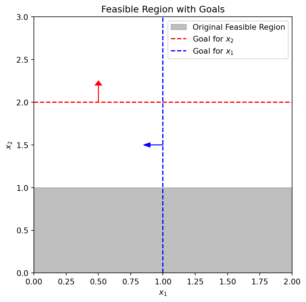
2. Assess the solution \((x_1, x_2) = (1, 1)\) with deficiency variables \(d_1^+ = 0\) and \(d_2^- = 1\). Is this solution considered Pareto efficient?

Question 3 - Answer

1. Goal Programming Model. Introduce deficiency variables \(d_1^+\) and \(d_2^-\) to measure how much \(x_1\) exceeds the goal of 1 and how much \(x_2\) is below the goal of 2, respectively.

\[ \begin{align*} \min &\quad d_1^+ + d_2^- \\ \text{s.t.} & \quad x_1 - d_1^+ \leq 1 \\ & \quad x_2 + d_2^- \geq 2 \\ & \quad 0 \leq x_1 \leq 2 \\ & \quad 0 \leq x_2 \leq 1 \\ & \quad d_1^+, d_2^- \geq 0 \end{align*} \]

2. Assessment of Pareto Efficiency. A solution is Pareto efficient if there is no way to make any one objective better off without making at least one objective worse off.

For the solution \((x_1, x_2) = (1, 1)\), with \(d_1^+ = 0\) and \(d_2^- = 1\):

• \(x_1\) meets the goal of not exceeding 1 without any deficiency.
• \(x_2\) does not meet the goal of being higher than 2; it is deficient by 1 unit.
• \(\min(d_1^+ + d_2^-) = 0 + 1 = 1\)

For this solution to be Pareto efficient, there cannot be any other feasible solution that would result in a better outcome for \(x_2\) without worsening \(x_1\).

However, for solution \((x_1, x_2) = (0, 1)\), we also have \(d_1^+ = 0\) and \(d_2^- = 1\):

• \(x_1\) meets the goal of not exceeding 1 without any deficiency.
• \(x_2\) does not meet the goal of being higher than 2; it is deficient by 1 unit.
• \(\min(d_1^+ + d_2^-) = 0 + 1 = 1\)

Therefore, the solution \((x_1, x_2) = (1, 1)\) is not Pareto efficient, as there exists another feasible solution \((0, 1)\) that is at least as good in one objective and better in the other.

Assuring Efficiency: By adding a small multiple of \(x_1\) (which was originally to be minimized) and subtracting a small multiple of \(x_2\) (which was originally to be maximized), we slightly shift the preference within the feasible region toward solutions that are better aligned with the original objectives.

This is a common technique in goal programming to assure that the solutions are efficient, meaning that they are as close as possible to the “ideal” solution that would be obtained if the original objectives could be fully achieved without any trade-offs. The new objective function aims to balance between minimizing the deficiencies and adhering to the original optimization:

\[ \begin{align*} \min &\quad d_1^+ + d_2^- +0.001x_1 - 0.001x_2 \\ \text{s.t.} & \quad x_1 - d_1^+ \leq 1 \\ & \quad x_2 + d_2^- \geq 2 \\ & \quad 0 \leq x_1 \leq 2 \\ & \quad 0 \leq x_2 \leq 1 \\ & \quad d_1^+, d_2^- \geq 0 \end{align*} \]

Question 4

Preemptive Goal Programming. A logistics company operates two types of automated guided vehicles (AGVs) within their warehouse: Type A and Type B. Each AGV has a different capacity for transporting goods and incurs different operating costs. The company aims to determine the optimal daily operational hours for both AGVs while adhering to the following set of hierarchical goals:

1. Cost Management (Priority 1): The total operational cost of utilizing both AGVs should not exceed €2000 per day.
2. Equitable Utilization (Priority 2): The daily working hours of vehicle A and vehicle B are the same.
3. Throughput Maximization (Priority 3): The company wants to transport as many pieces as possible per day.

Operational Parameters:

• Vehicle A: Transports 20 pieces per hour at a cost of €4 per piece.
• Vehicle B: Transports 30 pieces per hour at a cost of €3 per piece.
• Capacity Constraint: The company needs to move at least 250 pieces and no more than 600 pieces daily.

Develop a mathematical model to effectively address and satisfy these hierarchical priorities.

Question 4 - Answer

Note that we are dealing with a lexicographic goal programming problem. The first two priorities are associated with a goal (and hence deviations), whereas the last priority is to maximize the number of pieces transported. Therefore, we will initially address the problem of deviations and subsequently optimize the number of daily pieces transported, determining whether or not deviations are necessary. Finally, notice that this problem treated linearly.

Mathematical Model

• Decision Variables:

  • \(x_1\): Number of operating hours for vehicle A.
  • \(x_2\): Number of operating hours for vehicle B.

• Deficiency/Surplus Variables:

  • \(d_1^+\): Surplus variable for the total daily cost exceeding €2,000.
  • \(d_2^-\): Deficiency variable for the difference in daily working hours when vehicle A works less than vehicle B.
  • \(d_2^+\): Surplus variable for the difference in daily working hours when vehicle A works more than vehicle B.

• Objectives: We consider the following lexicographically ordered priorities:

  1. Minimize: \(f_1\) = \(d_1^+\) (Cost overrun)
     
  2. Minimize: \(f_2\) = \(d_2^- + d_2^+\) (Deviation from equitable utilization), considering optimal solutions for \(f_1\).
  3. Maximize: \(f_3\) = \(20x_1 + 30x_2\) (Throughput), considering optimal solutions for \(f_1\) and \(f_2\).

  This can be expressed as:

  \[ \min_L \big( f_1, f_2, -f_3 \big) \]

  where \(L\) denotes lexicographic ordering, ensuring strict priority among the objectives.

• Constraints:

  1. Minimum throughput: \(20x_1 + 30x_2 \geq 250\)
  2. Maximum capacity: \(20x_1 + 30x_2 \leq 600\)
  3. Maximum operational cost: \(80x_1 + 90x_2 - d_1^+ \leq 2000\)
  4. Equitable utilization of vehicles A and B: \(x_1 - x_2 - d_2^+ + d_2^- = 0\)
  5. Non-negativity: \(x_1, x_2, d_1^+, d_2^+, d_2^- \geq 0\)

Lexicographical Optimization

The solution to this warehouse optimization problem consists of three steps:

• 1) Minimize Cost Overrun (Priority 1). The optimal value of \(d_1^+\) will be the smallest non-negative number that satisfies the cost constraint. If the cost of operating both vehicles at their maximum capacity does not exceed €2,000, then \(d_1^+ = 0\). \[ \begin{align*} \min&\quad (d_1^+)\\ s.t.&\quad20x_1 + 30x_2 \geq 250 \\ &\quad20x_1 + 30x_2 \leq 600 \\ &\quad80x_1 + 90x_2 - d_1^+ \leq 2000 \\ &\quad x_1, x_2, d_1^+ \geq 0 \end{align*} \]

• 2) Ensure Equitable Utilization (Priority 2). With the cost constraint satisfied, the optimal values of \(d_2^-\) and \(d_2^+\) will be the smallest non-negative numbers that satisfy the equal hours constraint. In an ideal solution, both \(d_2^-\) and \(d_2^+\) will be zero, indicating perfect parity in operating hours (.e., \(x_1 = x_2\)). Notice that this constraint is an equality constraint, therefore, the solution has to be on the line. \[ \begin{align*} \min&\quad (d_2^- + d_2^+)\\ s.t.&\quad20x_1 + 30x_2 \geq 250 \\ &\quad20x_1 + 30x_2 \leq 600 \\ &\quad80x_1 + 90x_2 \leq 2,000 \\ &\quad x_1 - x_2 - d_2^+ + d_2^- = 0 \\ &\quad x_1, x_2, d_2^+, d_2^- \geq 0 \end{align*} \]

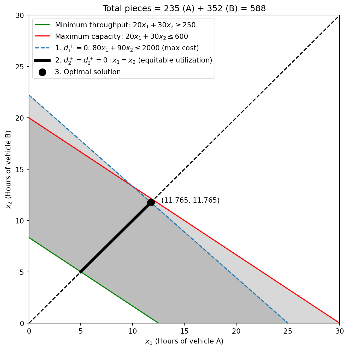
• Step 3: Maximize Throughput (Priority 3). Finally, with the cost and equitable utilization goals addressed, we aim to maximize the throughput, which is the total number of pieces moved. \[ \begin{align*} \max&\quad (20x_1 + 30x_2)\\ s.t.&\quad20x_1 + 30x_2 \geq 250 \\ &\quad20x_1 + 30x_2 \leq 600 \\ &\quad80x_1 + 90x_2 \leq 2,000 \\ &\quad x_1 - x_2 = 0 \\ &\quad x_1, x_2 \geq 0 \end{align*} \]

Solution

In the following, you can visualize the feasible region and the optimal solution for the lexicographic goal programming problem. Analyzing the solution, we found that both vehicles work 11.765 hours. There is an equilibrium between both vehicles as we can see that there is no deviation (\(d_2^+ = d_2^- = 0\)). So, a total of 235.3 and 352.95 pieces will be transported, that is, 235 and 352. With a total cost of 588.25 which is below 600 so there was no deviation from the goal \(d_1^+ = 0\).

Question 5

Goal Programming. Imagine you are tasked with optimizing the Vehicle Routing Problem (VRP) for your company, and the decision-maker (DM) has specified two key goals to guide your solution:

1. Vehicle Limitation: Use no more than three vehicles for the routing task.
2. Customer Arrival Time Window: Ensure that the arrival times at all customer locations are between 5 and 20 (inclusive).

Your challenge is to incorporate these goals into a goal programming model. How would you adjust the standard VRP formulation to accommodate these specific requirements? Modify the provided VRP model to align with the DM’s objectives.

Sets and Indices

• \(\mathcal{N}\): Set of all nodes (customers plus depot \(0\)).
• \(\mathcal{V}\): Set of vehicles available for routing.
• \(\mathcal{C}\): Set of customer nodes, where \(\mathcal{C} \subset \mathcal{N} \setminus \{0\}\).
• \(i, j\): Node indices, where \(i, j \in \mathcal{N}\).
• \(h\): Customer index, where \(h \in \mathcal{C}\).
• \(k\): Vehicle index, where \(k \in \mathcal{V}\).

Parameters

• \(c_{ij}\): Travel cost from node \(i\) to node \(j\), where \(i,j \in \mathcal{N}\).
• \(d_i\): Demand of customer at node \(i\), where \(i \in \mathcal{C}\).
• \(q\): Capacity of each vehicle in set \(\mathcal{V}\).
• \(t_{ij}\): Travel time from node \(i\) to node \(j\).

Variables

• \(x_{ijk}\): Binary variable indicating if vehicle \(k\) travels from node \(i\) to node \(j\).
• \(s_{ik}\): Arrival time at node \(i\) for vehicle \(k\).

VRP formulation

\[ \begin{align*} &&\min \sum_{k \in \mathcal{V}} \sum_{i \in \mathcal{N}} \sum_{j \in \mathcal{N}} c_{ij}x_{ijk} &&\label{eq:objective} \\ \end{align*} \]

\[ \begin{align*} &&\mathcal{s.t.} & & & \nonumber \\ &&\sum_{k \in \mathcal{V}}\sum_{j \in \mathcal{N}} x_{ijk} &= 1 && \forall i \in \mathcal{C}, \label{eq:customer_served} \\ &&\sum_{i \in \mathcal{C}} d_i \sum_{j \in \mathcal{N}} x_{ijk} &\leq q && \forall k \in \mathcal{V}, \label{eq:vehicle_capacity} \\ &&\sum_{j \in \mathcal{N}} x_{0jk} &= 1 && \forall k \in \mathcal{V}, \label{eq:depot_start} \\ &&\sum_{i \in \mathcal{N}} x_{ihk} - \sum_{j \in \mathcal{N}} x_{hjk} &= 0 && \forall h \in \mathcal{C}, \forall k \in \mathcal{V}, \label{eq:flow_conservation} \\ &&\sum_{i \in \mathcal{N}} x_{i,n+1,k} &= 1 && \forall k \in \mathcal{V}, \label{eq:depot_end} \\ &&x_{ijk}(s_{ik} + t_{ij} - s_{jk}) &\leq 0 && \forall i,j \in \mathcal{N}, \forall k \in \mathcal{V}, \label{eq:time_constraint} \\ &&x_{ijk} &\in \{0,1\} && \forall i, j \in \mathcal{N}, \forall k \in \mathcal{V}. \label{eq:binary_variables} \end{align*} \]

Non-Linearity Alert!

The time constraint \(x_{ijk}(s_{ik} + t_{ij} - s_{jk}) \leq 0\) introduces non-linearity in the model. In practice, you may need to linearize this constraint to ensure tractability or use a solver that can handle non-linear constraints.

Question 5 - Answer

1. Vehicle Limitation (Goal 1)

   • Standard (Hard) Constraint: This constraint ensures that no more than 3 vehicles leave the depot to serve customers.

     \[ \sum_{k \in \mathcal{V}}\sum_{j \in \mathcal{C}} x_{0jk} \leq 3 \]

   • Goal Constraint with Deficiency Variable \(d^+_1\): This constraint introduces a deficiency variable \(d^+_1\) to allow for flexibility in the vehicle limit. It measures the extent to which the solution exceeds the preferred limit of 3 vehicles.

     \[ \sum_{k \in \mathcal{V}}\sum_{j \in \mathcal{C}} x_{0jk} - d^+_1 \leq 3 \]

2. Customer Arrival Time Window (Goal 2)

   • Standard (Hard) Constraints: These constraints ensure that the arrival times at each customer node \(i\) by any vehicle \(k\) are no earlier than 5 and no later than 20.

     \[ s_{ik} \geq 5 \quad \forall i \in \mathcal{C}, \forall k \in \mathcal{V} \] \[ s_{ik} \leq 20 \quad \forall i \in \mathcal{C}, \forall k \in \mathcal{V} \]

   • Goal Constraints with Deficiency Variables \(d_{2ik}^+\) and \(d_{2ik}^-\): These constraints introduce deficiency variables to manage deviations from the desired arrival time window. \(d_{2ik}^-\) captures the underachievement (arrival too early), while \(d_{2ik}^+\) captures overachievement (arrival too late).

     \[ s_{ik} +d_{2ik}^- \geq 5 \quad \forall i \in \mathcal{C}, \forall k \in \mathcal{V} \] \[ s_{ik} -d_{2ik}^+ \leq 20 \quad \forall i \in \mathcal{C}, \forall k \in \mathcal{V} \]

Objective Function Alternatives

Many objective function configurations are possible, such as weigthed scoring and lexicographical.

1. Weighted Scoring Objective Function

   This objective function balances the total travel cost against the fulfillment of specific goals (vehicle limit and customer arrival time window). It combines these aspects into a single expression, weighted to reflect their relative importance:

   \[ \min \left( \sum_{k \in \mathcal{V}} \sum_{i \in \mathcal{N}} \sum_{j \in \mathcal{N}} c_{ij}x_{ijk} + \alpha_1 d^+_1 + \alpha_2 \sum_{i \in \mathcal{C}} \sum_{k \in \mathcal{V}} (d_{2ik}^+ + d_{2ik}^-) \right) \]

   • The first term minimizes the total travel cost.
   • The second term \(\alpha_1 d^+_1\) represents the weighted penalty for exceeding the maximum number of vehicles.
   • The third term \(\alpha_2 \sum (d_{2ik}^+ + d_{2ik}^-)\) is the weighted sum of deviations from the desired arrival times at customer locations.
   • Weights \(\alpha_1\) and \(\alpha_2\) indicate the relative importance of each goal compared to the cost.

2. Lexicographical Objective Function

   In this approach, the primary focus is on minimizing the sum of all deficiency variables before considering the travel cost. This ensures adherence to the decision-maker’s goals is prioritized:

   • First Stage: Minimize total deficiencies.

     \[ \min \left( \alpha_1 d^+_1 + \alpha_2 \sum_{i \in \mathcal{C}} \sum_{k \in \mathcal{V}} (d_{2ik}^+ + d_{2ik}^-) \right) \]

     • \(\alpha_1 d^+_1\) and \(\alpha_2 \sum (d_{2ik}^+ + d_{2ik}^-)\) represent the total deficiencies related to the vehicle limit and arrival times, respectively.

   • Second Stage: After minimizing deficiencies, minimize the total travel cost.

     \[ \min \sum_{k \in \mathcal{V}} \sum_{i \in \mathcal{N}} \sum_{j \in \mathcal{N}} c_{ij}x_{ijk} \]

Question 6

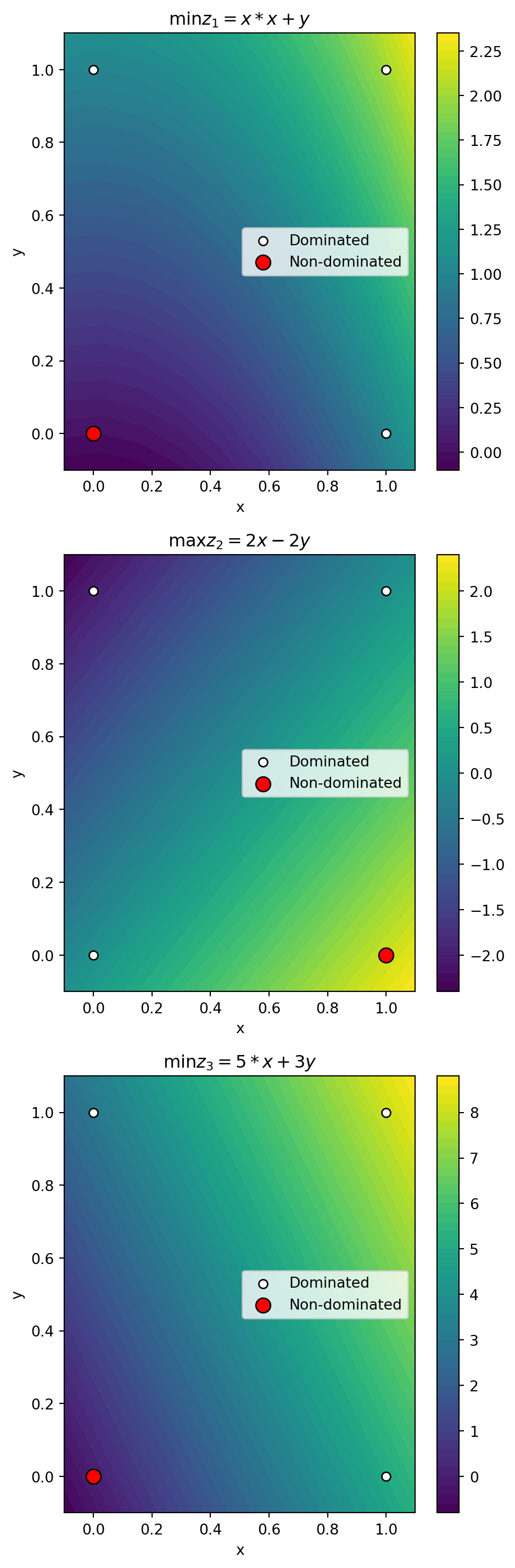
Pareto Dominance. Consider the following objective functions:

1. \(\min z_1 = x*x + y\)
2. \(\max z_2 = 2x - 2y\)
3. \(\min z_3 = 5*x + 3y\)

Given the solutions:

• (0,0)
• (0,1)
• (1,0)
• (1,1)

Determine which solutions are dominated and which are not, according to each objective function.

Question 6 - Answer

The values for each solution according to the objective functions are as follows:

Table 1: Table 1: Objective function values for each solution across three objectives.

Solution	\(\min z_1 = x*x + y\)	\(\max z_2 = 2x - 2y\)	\(\min z_3 = 5x + 3y\)
(0,0)	0	0	0
(0,1)	1	-2	3
(1,0)	1	2	5
(1,1)	2	0	8

Analysis:

1. For \(\min z_1 = x*x + y\), the non-dominated solution is (0,0) with the value 0.
2. For \(\max z_2 = 2x - 2y\), the non-dominated solution is (1,0) with the value 2.
3. For \(\min z_3 = 5x + 3y\), the non-dominated solution is (0,0) with the value 0.

Question 7

Selecting Suppliers with Analytical Hierarchy Process (AHP). Your company wants to select a new wheels supplier using AHP. It has two possible companies (i.e., R3 and Brock). The decision hierarchy is as follows:

• Goal: Choose a new wheels supplier
• Criteria:
  • Cost
  • Quality
  • Delivery
• Alternatives:
  • R3
  • Brock

Consider that managerial judgments are quantifyied using the pairwise comparison matrix below.

Table 2: Pairwise comparison scale for AHP.

Verbal judgment or preference	Numerical rating
Extremely preferred	9
Very strongly preferred	7
Strongly preferred	5
Moderately preferred	3
Equally preferred	1
Intermediate values between two adjacent judgments (when compromise is needed)	2, 4, 6, and 8

Using these ratings, consider management has evaluated three criteria: cost, quality, and delivery as follows:

Table 3: Pairwise comparison matrix for the criteria.

Criteria	Cost	Quality	Delivery
Cost	1	7	3
Quality	1/7	1	1/3
Delivery	1/3	3	1

Before choosing the supplier, calculate the consistency ratio of the evaluation criteria.

Question 7 - Answer

Calculating the consistency ratio (CR) for the evaluations involves the following steps.

1. Normalize the Pairwise Comparison Matrix:

   • First, create the pairwise comparison matrix:

   	Cost	Quality	Delivery
   Criteria
   Cost	1.00	7.0	3.00
   Quality	0.14	1.0	0.33
   Delivery	0.33	3.0	1.00

   The corresponding positions below the diagonals are the reciprocals of the judgments already entered. Assuming as before that the pairwise comparison of cost to delivery is 3, or equivalently a 3 to 1 ratio, it follows that the pairwise comparison of delivery to cost is a 1 to 3 ratio, or 1/3.

   Note

   Reciprocals: If activity \(i\) has a specific numerical rating with respect to activity \(j\), then \(j\) has the reciprocal value when compared to \(i\).

   • Then, normalize this matrix by dividing each element by the sum of its column.

   	Cost	Quality	Delivery
   Criteria
   Cost	0.68	0.64	0.69
   Quality	0.10	0.09	0.08
   Delivery	0.23	0.27	0.23

2. Compute the Priority Vector:

   • Calculate the priority vector by averaging the rows of the normalized matrix.

   The final weights are: {'Cost': 0.669, 'Quality': 0.088, 'Delivery': 0.243}

   	Cost	Quality	Delivery	priority
   Criteria
   Cost	1.00	7.0	3.00	0.67
   Quality	0.14	1.0	0.33	0.09
   Delivery	0.33	3.0	1.00	0.24

   Therefore, cost is judged to be about 7.60 times (0.669/0.088) as important as quality and about 2.75 times (0.669/0.243) as important as delivery.

   Note

   One important advantage of using AHP is that it can measure the degree to which a manager’s judgments are consistent.

3. Calculate the Weighted Sum Vector:

   • Multiply each element of the original matrix by the corresponding element in the priority vector.

   	Cost	Quality	Delivery
   Criteria
   Cost	0.668697	0.617415	0.729303
   Quality	0.095528	0.088202	0.081034
   Delivery	0.222899	0.264606	0.243101

   • Sum each column to get the weighted sum vector.

   	Cost	Quality	Delivery	Sum
   Criteria
   Cost	0.669	0.617	0.729	2.015
   Quality	0.096	0.088	0.081	0.265
   Delivery	0.223	0.265	0.243	0.731

4. Determine the Largest Eigenvalue \(\lambda_{\text{max}}\):

   • Divide each value in the “Sum” column by the priority weight of its corresponding criterion. This step normalizes the weighted sum vector with respect to the priority weights leading to what is called the consistency vector.

   	Consistency
   Criteria
   Cost	3.013944
   Quality	3.001786
   Delivery	3.005361

   Note

   Ideally, if the comparisons are perfectly consistent, all the elements of the consistency vector should be equal to \(\lambda_{\text{max}}\) since the priority vector is the true eigenvector associated with \(\lambda_{\text{max}}\).

   • Compute the largest Eigenvalue from the weighted sum vector and priority vector.

   Largest Eigenvalue: 3.007

   Note

   The average of the values obtained by dividing the elements of the weighted sum vector by the corresponding elements of the priority vector is used as an approximation for the maximum eigenvalue (\(\lambda_{max}\)) of the pairwise comparison matrix.

5. Derive the Consistency Index (CI):

   • Use the formula \(CI = \frac{\lambda_{\text{max}} - n}{n - 1}\), where \(n\) is the number of criteria.

   
   Consistency Index (CI): 0.004

6. Consult Saaty’s Random Index (RI) Table:

   • Use the RI value corresponding to the matrix size from Saaty’s table.

     n	3	4	5	6
     RI	0.58	0.9	1.12	1.24

     For a 3x3 matrix, the RI is 0.58.

7. Calculate the Consistency Ratio (CR):

   • Use \(CR = \frac{CI}{RI}\).

   
   Consistency Ratio (CR): 0.006

Result: A CR value of 0.10 or less indicates acceptable consistency in the decision-making process. If CR exceeds 0.10, the judgments may need reevaluation. Therefore, decision-making process AHP can continue.

Question 8

Preemptive Goal Programming. Logistics Innova plans to assemble two new product scanners, KS500 and KS600, each requiring the same type of plastic frame and optical scanners. The KS500 needs 2 optical scanners, while the KS600 requires an optical scanner and a card reader. Weekly availability includes 1000 optical scanners, 500 card scanners, and 600 plastic frames. Assembling a KS500 takes 1 hour and yields a 200 euro benefit, whereas the KS600 takes 1.5 hours and provides a 500 euro benefit. The company’s goals, in order of priority, are:

1. Produce at least 200 KS500 scanners weekly.
2. Assemble a minimum of 500 scanners in total per week.
3. Equalize total work hours for both scanner types.
4. Achieve a weekly benefit of at least 250,000 euros.

Determine and interpret the optimal solution for these objectives.

Question 8 - Answer

The deviation for priority 4 (weekly benefit goal) is 58,000 euros, indicating a shortfall from the target. For priorities 1 to 3, which involve production targets and work hour balancing, the deviation is zero (these goals are fully met). The optimal solution for the scanner production is assembling 360 units of KS500 and 240 units of KS600.

References

Lexicographic Method

The lexicographic method is an optimization approach that prioritizes objective functions based on their importance, rather than assigning numerical weights or aggregating them into a single function. Instead of normalizing objectives or balancing trade-offs, this method ranks them in strict order and optimizes them sequentially.

Mathematical Representation

Consider a problem with \(q\) objective functions, \(f_1(x), f_2(x), \dots, f_q(x)\), ranked in decreasing order of priority. The lexicographic optimization problem is formulated as:

\[ \min_{x \in S} f_i(x) \]

Subject to: \[ f_j(x) \leq f_j(x^*) \quad \forall j = 1, \dots, i-1, \quad i = 1, \dots, q \]

where:
- \(S\) represents the feasible solution set.
- \(x^*\) denotes the optimal solution found at each previous step.
- The constraints ensure that each subsequent objective is optimized without degrading the optimality of higher-priority objectives.

This iterative process guarantees that the final solution is always Pareto optimal, meaning that no objective can be improved without worsening a higher-priority one.

Advantages

1. Unique preference specification: It allows for strict priority-based decision-making.
   
2. No need for normalization: Unlike weighted sum methods, objectives do not have to be scaled.
   
3. Guaranteed Pareto optimality: The final solution is always Pareto optimal, ensuring no unnecessary trade-offs.

Disadvantages

1. Computationally expensive: Solving multiple single-objective problems can be demanding, especially for large-scale problems.
   
2. Constraint growth: As objectives are sequentially optimized, additional constraints are imposed, leading to a large constraint set when many objectives are considered.
   
3. A-priori preference setup: In some cases, it is difficult to define preferences a priori, especially when multiple objectives are of similar importance or interact in complex ways. Presenting a pallete of solutions can be more informative, as it allows decision-makers to explore trade-offs.