Practice Exercises - Mathematical Modeling

Question 1

Customizing a VRP. Given the Vehicle Routing Problem (VRP) model below, implement the necessary modifications to the constraints and objective function to accommodate the following enhancements:

1. Incorporating Time Windows: How would you modify the VRP model to include time windows for each customer, ensuring that each customer is served within a specific time frame?
2. Limiting the Fleet Size: What changes would you make to the VRP model to incorporate a constraint on the maximum number of vehicles that can be used in the routing plan?
3. Minimizing Waiting Times: How would you change the formulation to include the minimization of waiting times as an objective to optimize?

Sets and Indices

• \(\mathcal{N}\): Set of all nodes (customers plus depot \(0\)).
• \(\mathcal{V}\): Set of vehicles available for routing.
• \(\mathcal{C}\): Set of customer nodes, where \(\mathcal{C} \subset \mathcal{N} \setminus \{0\}\).
• \(i, j\): Node indices, where \(i, j \in \mathcal{N}\).
• \(h\): Customer index, where \(h \in \mathcal{C}\).
• \(k\): Vehicle index, where \(k \in \mathcal{V}\).

Parameters

• \(c_{ij}\): Travel cost from node \(i\) to node \(j\), where \(i,j \in \mathcal{N}\).
• \(d_i\): Demand of customer at node \(i\), where \(i \in \mathcal{C}\).
• \(q\): Capacity of each vehicle in set \(\mathcal{V}\).
• \(t_{ij}\): Travel time from node \(i\) to node \(j\).

Variables

• \(x_{ijk}\): Binary variable indicating if vehicle \(k\) travels from node \(i\) to node \(j\).
• \(s_{ik}\): Arrival time at node \(i\) for vehicle \(k\).

VRP formulation

\[\begin{align} &&\min \sum_{k \in \mathcal{V}} \sum_{i \in \mathcal{N}} \sum_{j \in \mathcal{N}} c_{ij}x_{ijk} &&\label{eq:objective} \\ \end{align}\] \[\begin{align} &&\mathcal{s.t.} & & & \nonumber \\ &&\sum_{k \in \mathcal{V}}\sum_{j \in \mathcal{N}} x_{ijk} &= 1 && \forall i \in \mathcal{C}, \label{eq:customer_served} \\ &&\sum_{i \in \mathcal{C}} d_i \sum_{j \in \mathcal{N}} x_{ijk} &\leq q && \forall k \in \mathcal{V}, \label{eq:vehicle_capacity} \\ &&\sum_{j \in \mathcal{N}} x_{0jk} &= 1 && \forall k \in \mathcal{V}, \label{eq:depot_start} \\ &&\sum_{i \in \mathcal{N}} x_{ihk} - \sum_{j \in \mathcal{N}} x_{hjk} &= 0 && \forall h \in \mathcal{C}, \forall k \in \mathcal{V}, \label{eq:flow_conservation} \\ &&\sum_{i \in \mathcal{N}} x_{i,n+1,k} &= 1 && \forall k \in \mathcal{V}, \label{eq:depot_end} \\ &&x_{ijk}(s_{ik} + t_{ij} - s_{jk}) &\leq 0 && \forall i,j \in \mathcal{N}, \forall k \in \mathcal{V}, \label{eq:time_constraint} \\ &&x_{ijk} &\in \{0,1\} && \forall i, j \in \mathcal{N}, \forall k \in \mathcal{V}. \label{eq:binary_variables} \end{align}\]

Solution 1

1. Incorporating Time Windows

To include time windows for each customer, we need to define the additional parameters:

• \(e_i\): Earliest start time for serving customer at node \(i\).
• \(l_i\): Latest start time for serving customer at node \(i\).

Then, we can add a time window constraint to esure each customer is served within their specific time frame:

\[ e_i \leq s_{ik} \leq l_i \quad \forall i \in \mathcal{C}, \forall k \in \mathcal{V} \]

And update the time constraint:

\[ s_{ik} + t_{ij} - s_{jk} \leq M(1 - x_{ijk}) \quad \forall i, j \in \mathcal{N}, \forall k \in \mathcal{V} \]

Where \(M\) is a large constant.

2. Limiting the Fleet Size

To limit the fleet size, we add a new constraint on the maximum number of vehicles used \(K_{\text{max}}\):

\[ \sum_{k \in \mathcal{V}} y_k \leq K_{\text{max}} \]

Where \(y_k\) is a binary variable indicating if vehicle \(k\) is used. To connect the use of a vehicle \(k\) (\(y_k\)) to its routing decisions (\(x_{ijk}\)), we consider that if a vehicle is used (\(y_k = 1\)), it must leave from and return to the depot. If a vehicle is not used (\(y_k = 0\)), it cannot leave from or return to the depot.

\[ \sum_{j \in \mathcal{N}} x_{0jk} = y_k \quad \forall k \in \mathcal{V} \]

\[ \sum_{i \in \mathcal{N}} x_{i,n+1,k} = y_k \quad \forall k \in \mathcal{V} \]

Note

In this model, we consider that each vehicle can only have at most one trip assigned to it, starting and ending at the depot. In some VRP settings, vehicles can be required to do many trips back and forth from the depot (see the multi-trip VRP by Brandão and Mercer 1998).

3. Minimizing Waiting Times

To minimize waiting times, we can adjust the objective function to include a penalty for waiting \(w_{ik}\) (waiting at node \(i\) for vehicle \(k\)).

Then, we can add a term to the objective function to minimize waiting times, weighted by a penalty factor \(\alpha\):

\[ \min \sum_{k \in \mathcal{V}} \sum_{i \in \mathcal{N}} \sum_{j \in \mathcal{N}} c_{ij}x_{ijk} + \alpha \sum_{k \in \mathcal{V}} \sum_{i \in \mathcal{C}} w_{ik} \]

Waiting times are calculated using a constraint as the difference between arrival times and earliest start times:

\[ w_{ik} \geq e_i - s_{ik} \quad \forall i \in \mathcal{C}, \forall k \in \mathcal{V} \]

Validation:

Considering the following problem input:

• Nodes: [0, 1, 2, 3, 4, 5]

• Customers: [1, 2, 3, 4]

• Demands: [0, 1, 2, 3, 4, 0]

• Earliest arrival times: [0, 0, 0, 0, 0, 0]

• Latest arrival times: [inf, 100, 100, 100, 100, inf]

• Vehicles: [1, 2, 3]

• Vehicles’ capacity: 10

• Max. fleet size: 3

• Weight for waiting times \(\alpha\): 0.5

And assuming 10-unit travel times, as shown in Table 1:

Table 1: Travel times. The first and last nodes represent start and end depots.

	0	1	2	3	4	5
0	0	10	10	10	10	0
1	10	0	10	10	10	10
2	10	10	0	10	10	10
3	10	10	10	0	10	10
4	10	10	10	10	0	10
5	0	10	10	10	10	0

We have the following results:

s_1_1 = 10.0
s_2_3 = 10.0
s_3_3 = 20.0
s_4_1 = 20.0
s_5_1 = 30.0
s_5_3 = 30.0
w_1_1 = 10.0
w_2_3 = 10.0
w_3_3 = 20.0
w_4_1 = 20.0
w_5_1 = 30.0
w_5_3 = 30.0
x_0_1_1 = 1.0
x_0_2_3 = 1.0
x_1_4_1 = 1.0
x_2_3_3 = 1.0
x_3_5_3 = 1.0
x_4_5_1 = 1.0
y_1 = 1.0
y_3 = 1.0
Total cost = 120.0

Vehicle 1:

• Route: [0, 1, 4, 5]

• Arrivals: [0.0, 10.0, 20.0, 30.0]

• Waitings: [0.0, 10.0, 20.0, 30.0]

Vehicle 2:

• Route: [0]

• Arrivals: [0.0]

• Waitings: [0.0]

Vehicle 3:

• Route: [0, 2, 3, 5]

• Arrivals: [0.0, 10.0, 20.0, 30.0]

• Waitings: [0.0, 10.0, 20.0, 30.0]

Question 2

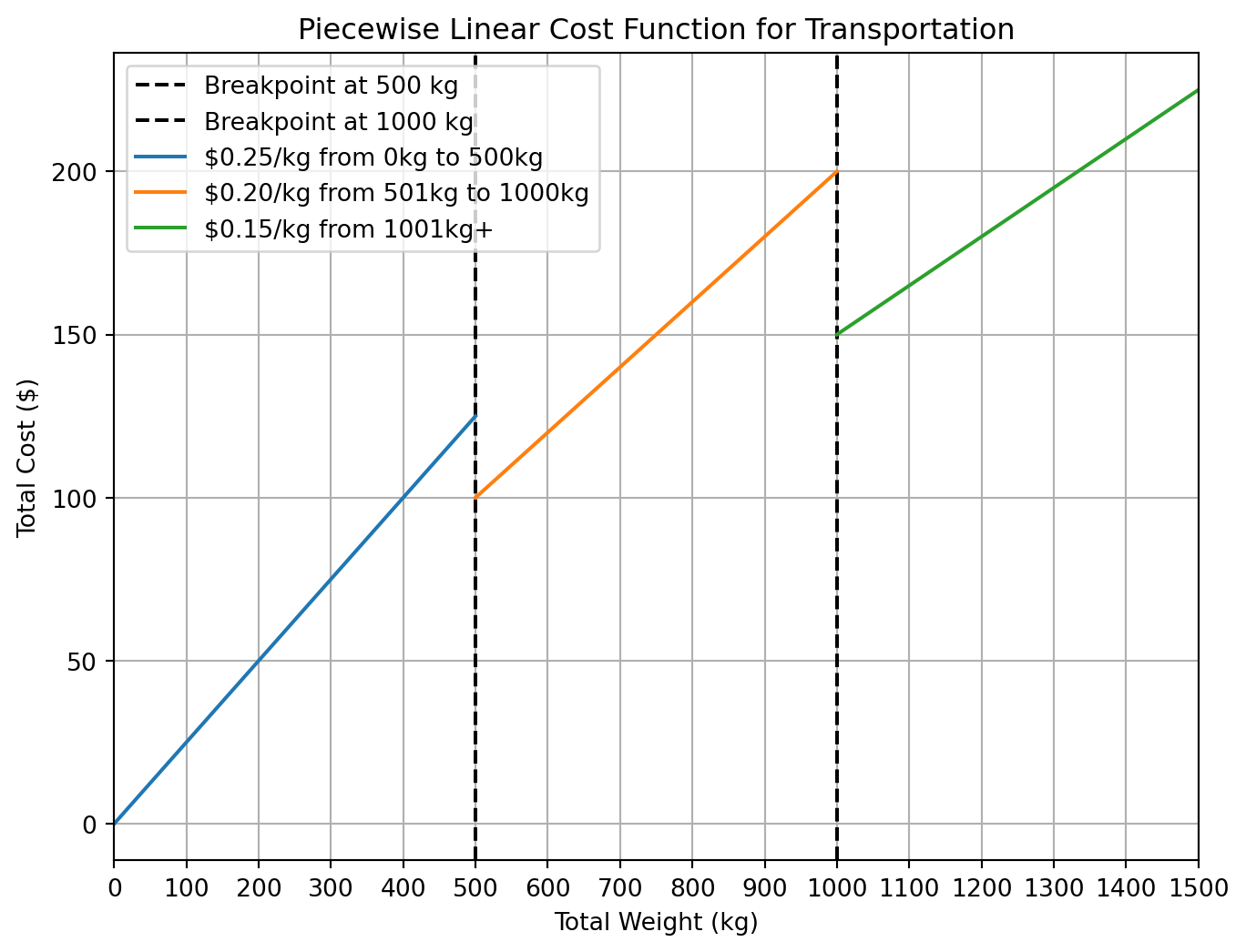
Piecewise Linear Costs. Ongoing Logistics offers two truck services, Truck Service 1 and Truck Service 2, which transport bulk material and pallet loads (measured in kilograms). For each kilogram transported by Truck Service 1, at least 50% must be bulk material. Meanwhile, for each kilogram transported by Truck Service 2, at least 60% must be bulk material. Using Truck Service 1 yields a profit of 20 cents per kilogram, whereas Truck Service 2 generates a profit of 24 cents per kilogram. There is a need to transport 1,000 kilograms of bulk and 500 kilograms of pallets. Truck Service 1 has a capacity limit of 900 kilograms, and Truck Service 2 has a limit of 700 kilograms.

The transportation costs are as follows:

• Up to 500 kilograms cost 25 cents per kilogram;
• The next 500 kilograms cost 20 cents per kilogram; and
• Any amount above that costs 15 cents per kilogram.

Formulate a model to maximize Ongoing Logistics’ profits.

Solution 2

Decision Variables

• \(x^{\text{S1}}_{\text{bulk}}\): Kilograms of bulk material transported by Truck Service 1.
• \(x^{\text{S2}}_{\text{bulk}}\): Kilograms of bulk material transported by Truck Service 2.
• \(x^{\text{S1}}_{\text{pallet}}\): Kilograms of pallets transported by Truck Service 1.
• \(x^{\text{S2}}_{\text{pallet}}\): Kilograms of pallets transported by Truck Service 2.
• \(y_{\text{1}}, y_{\text{2}}, y_{\text{3}}\): Total load under cost segments 1 (0kg–500kg), 2 (501kg–1000kg), and 3 (higher than 1000kg), respectively.
• \(b_1, b_2, b_3\): Binary variables representing the activation of different cost segments.
  • If \(b_1 = 1\), the total load is between 0 and 500.
  • If \(b_2 = 1\), the total load is between 501 and 1000.
  • If \(b_3 = 1\), the total load exceeds 1000.

Objective Function

\[ \max 0.20 (x_{\text{bulk}}^{\text{S1}} + x_{\text{pallet}}^{\text{S1}}) + 0.24 (x_{\text{bulk}}^{\text{S2}} + x_{\text{pallet}}^{\text{S2}}) - (0.25 y_1 + 0.20 y_2 + 0.15 y_3) \]

The cost function is as follows:

Constraints

• Truck Service Capacity:
  • Truck Service 1: \(x_{\text{bulk}}^{\text{S1}} + x_{\text{pallet}}^{\text{S1}} \leq 900\)
  • Truck Service 2: \(x_{\text{bulk}}^{\text{S2}} + x_{\text{pallet}}^{\text{S2}} \leq 700\)
• Material Demand Fulfillment:
  • Bulk Material: \(x_{\text{bulk}}^{\text{S1}} + x_{\text{bulk}}^{\text{S2}} = 1000\)
  • Pallet Load: \(x_{\text{pallet}}^{\text{S1}} + x_{\text{pallet}}^{\text{S2}} = 500\)
• Minimum Bulk Material Requirement for Each Truck:
  • Truck 1: \(x_{\text{bulk}}^{\text{S1}} \geq 0.5 (x_{\text{bulk}}^{\text{S1}} + x_{\text{pallet}}^{\text{S1}})\)
  • Truck 2: \(x_{\text{bulk}}^{\text{S2}} \geq 0.6 (x_{\text{bulk}}^{\text{S2}} + x_{\text{pallet}}^{\text{S2}})\)
• Total Load Calculation:
  • \(x_{\text{total}} = x_{\text{bulk}}^{\text{S1}} + x_{\text{bulk}}^{\text{S2}} + x_{\text{pallet}}^{\text{S1}} + x_{\text{pallet}}^{\text{S2}}\)
• Cost Segments Activation:
  • \(y_1 + y_2 + y_3 = x_{\text{total}}\)
  • \(b_1 + b_2 + b_3 = 1\)
• Cost Segment Boundaries (Big-M Constraints):
  • \(x_{\text{total}} \leq 500 - M (b_1 - 1)\)
  • \(x_{\text{total}} \geq 501 + M (b_2 - 1)\)
  • \(x_{\text{total}} \leq 1000 - M (b_2 - 1)\)
  • \(x_{\text{total}} \geq 1001 + M (b_3 - 1)\)
• Load Distribution within Cost Segments:
  • \(y_1 \geq x_{\text{total}} - M (1 - b_1)\)
  • \(y_1 \leq 500 (b_2 + b_3)\)
  • \(y_2 \geq x_{\text{total}} - y_1 - M (1 - b_2)\)
  • \(y_2 \leq 500 b_3\)
  • \(y_3 \geq x_{\text{total}} - y_2 - y_1 - M (1-b3)\)

Validation

We perform boundary tests to validate the model to check whether the correct segments are selected when the total load is at the extreme ends of the breakpoints.

Test 1 - Original input - Total load=1500 (Cost segment 3)

• Input
  • capacity_s1 = 900
  • capacity_s2 = 700
  • bulk = 1000
  • pallet = 500
• Results
  • Profit = 28
  • \(x_{bulk}^{S1}\) = 580
  • \(x_{bulk}^{S2}\) = 420
  • \(x_{pallet}^{S1}\) = 220
  • \(x_{pallet}^{S2}\) = 280
  • \(x_{total}\) = 1500
  • \(y_1\) = 500
  • \(y_2\) = 500
  • \(y_3\) = 500
  • \(b_1\) = 0
  • \(b_2\) = 0
  • \(b_3\) = 1

Test 2 - Total load=500 (Cost segment 1)

• Input
  • capacity_s1 = 250
  • capacity_s2 = 250
  • bulk = 400
  • pallet = 100
• Results
  • Profit = -15
  • \(x_{bulk}^{S1}\) = 150
  • \(x_{bulk}^{S2}\) = 250
  • \(x_{pallet}^{S1}\) = 100
  • \(x_{pallet}^{S2}\) = 0
  • \(x_{total}\) = 500
  • \(y_1\) = 500
  • \(y_2\) = 0
  • \(y_3\) = 0
  • \(b_1\) = 1
  • \(b_2\) = 0
  • \(b_3\) = 0

Test 3 - Total load=501 (Cost segment 2)

• Input
  • capacity_s1 = 251
  • capacity_s2 = 250
  • bulk = 401
  • pallet = 100
• Results
  • Profit = -15.00
  • \(x_{bulk}^{S1}\) = 151
  • \(x_{bulk}^{S2}\) = 250
  • \(x_{pallet}^{S1}\) = 100
  • \(x_{pallet}^{S2}\) = 0
  • \(x_{total}\) = 501
  • \(y_1\) = 500
  • \(y_2\) = 1
  • \(y_3\) = 0
  • \(b_1\) = 0
  • \(b_2\) = 1
  • \(b_3\) = 0

Test 4 - Total load=600 (Cost segment 2)

• Input
  • capacity_s1 = 300
  • capacity_s2 = 300
  • bulk = 400
  • pallet = 200
• Results
  • Profit = -13
  • \(x_{bulk}^{S1}\) = 220
  • \(x_{bulk}^{S2}\) = 180
  • \(x_{pallet}^{S1}\) = 80
  • \(x_{pallet}^{S2}\) = 120
  • \(x_{total}\) = 600
  • \(y_1\) = 500
  • \(y_2\) = 100
  • \(y_3\) = 0
  • \(b_1\) = 0
  • \(b_2\) = 1
  • \(b_3\) = 0

Test 5 - Total load=1000 (Cost segment 2)

• Input
  • capacity_s1 = 500
  • capacity_s2 = 500
  • bulk = 700
  • pallet = 300
• Results
  • Profit = -5
  • \(x_{bulk}^{S1}\) = 400
  • \(x_{bulk}^{S2}\) = 300
  • \(x_{pallet}^{S1}\) = 100
  • \(x_{pallet}^{S2}\) = 200
  • \(x_{total}\) = 1000
  • \(y_1\) = 500
  • \(y_2\) = 500
  • \(y_3\) = 0
  • \(b_1\) = 0
  • \(b_2\) = 1
  • \(b_3\) = 0

Test 6 - Total load=1001 (Cost segment 3)

• Input
  • capacity_s1 = 501
  • capacity_s2 = 500
  • bulk = 701
  • pallet = 300
• Results
  • Profit = -4.95
  • \(x_{bulk}^{S1}\) = 401
  • \(x_{bulk}^{S2}\) = 300
  • \(x_{pallet}^{S1}\) = 100
  • \(x_{pallet}^{S2}\) = 200
  • \(x_{total}\) = 1001
  • \(y_1\) = 500
  • \(y_2\) = 500
  • \(y_3\) = 1
  • \(b_1\) = 0
  • \(b_2\) = 0
  • \(b_3\) = 1

Question 3

Air-Cargo Transportation Load Planning. An air-cargo transportation company needs to load cargo onto two airplanes, each with three compartments for storage: front, center, and rear. The weight and space capacities of these compartments are provided in Table 2. There are four types of cargoes available for shipment on the next flight(s), as shown in Table 3. Cargo can be divided as needed among airplanes. Using an airplane incurs a one-time utilization cost, as detailed in Table 4.

Propose a mixed integer linear programming (MILP) model to solve this problem so that the total profit is maximized while respecting the weight and space capacities of each compartment and minimizing the airplane usage costs.

Your model should determine:

1. How many airplanes should be used.
2. How much of each cargo type should be accepted.
3. How to distribute the accepted cargo among the compartments of the airplanes to maximize the total profit.

Table 2: Weight and space capacities of airplane storage compartments.

Compartment	Weight Capacity (tonnes)	Space Capacity (cubic meters)
Front	10	6800
Center	16	8700
Rear	8	5300

Table 3: Types of cargoes available for shipment.

Type of Cargo	Total Amount (tonnes)	Volume (cubic meters/tonne)	Profit (€/tonne)
C1	18	480	310
C2	15	650	380
C3	23	580	350
C4	22	380	285

Table 4: The cost to use an airplane in euros.

Airplane	Utilization Cost (€)
A1	5000
A2	5000

Solution 3

Sets and Indices

• \(I = \{\text{Front} , \text{Center}, \text{Rear}\}\): Set of compartment type indices.
• \(C = \{\text{C1}, \text{C2}, \text{C3}, \text{C4}\}\): Set of cargo type indices.
• \(A = \{\text{A1}, \text{A2}\}\): Set of airplane indices.

Parameters

• \(w_i\): Weight capacity of compartment \(i\) in tonnes.
• \(s_i\): Space capacity of compartment \(i\) in cubic meters.
• \(\alpha^{\text{amount}}_c\): Total amount available of cargo type \(c\) in tonnes.
• \(\alpha^{\text{volume}}_c\): Volume per tonne for cargo type \(c\) in cubic meters/tonne.
• \(\alpha^{\text{profit}}_c\): Profit per tonne for cargo type \(c\) in euros.
• \(C\): Cost to use an airplane in euros.

Variables

• \(x_{ica}\): Amount of cargo type \(c\) loaded in compartment type \(i\) of airplane \(a\) in tonnes.
• \(y_a\): Binary variable indicating if airplane \(a\) is used (1 if used, 0 otherwise).

Objective Function

Maximize the total profit from transporting the cargo minus the cost of using the airplanes.

\(\displaystyle \max Z = \sum_{c \in C} \alpha^{\text{profit}}_c \sum_{i \in I} \sum_{a \in A} x_{ica} - C \sum_{a \in A} y_a\)

Constraints

1. Weight Capacity: The total cargo weight in each airplane compartment must not exceed its weight capacity. \[ \sum_{c \in C} x_{ica} \leq w_i y_a \quad \forall i \in I, a \in A \]

2. Space Capacity: The total cargo volume in each airplane compartment must not exceed its space capacity. \[ \sum_{c \in C} \alpha^{\text{volume}}_c x_{ica} \leq s_i y_a \quad \forall i \in I, a \in A \]

3. Cargo Availability: The amount of each cargo type used cannot exceed its available amount. \[ \sum_{i \in I} \sum_{a \in A} x_{ica} \leq \alpha^{\text{amount}}_c \quad \forall c \in C \]

4. Non-Negativity and Integrality: The amounts of cargo loaded must be non-negative, and the use of airplanes is a binary decision. \[ x_{ica} \geq 0 \quad \forall i \in I, c \in C, a \in A \\ y_a \in \{0, 1\} \quad \forall a \in A \]

Validation

We show the distribution of cargo across the compartments, considering different airplane usage costs:

• Airplane Usage Cost = 5,000 (Profit = 12,750.00)

			Weight (tonnes)	Volume (cubic meters)	Airplane Used	Revenue
Airplane	Compartment	Cargo Type
A1	Center	C1	5.0	2400.0	1	1550.0
		C2	7.9	5103.7	1	2983.7
		C4	3.1	1196.3	1	897.2
		Empty Center	0.0	0.0	1	0.0
	Front	C1	3.0	1440.0	1	930.0
		C3	7.0	4060.0	1	2450.0
		Empty Front	0.0	1300.0	1	0.0
	Rear	C3	8.0	4640.0	1	2800.0
		Empty Rear	0.0	660.0	1	0.0
A2	Center	C2	7.1	4646.3	1	2716.3
		C4	8.9	3363.7	1	2522.8
		Empty Center	0.0	690.0	1	0.0
	Front	C1	10.0	4800.0	1	3100.0
		Empty Front	0.0	2000.0	1	0.0
	Rear	C3	8.0	4640.0	1	2800.0
		Empty Rear	0.0	660.0	1	0.0

• Airplane Usage Cost = 10,000 (Profit = 2,750.00)

			Weight (tonnes)	Volume (cubic meters)	Airplane Used	Revenue
Airplane	Compartment	Cargo Type
A1	Center	C1	2.0	960.0	1	620.0
		C2	9.0	5825.9	1	3405.9
		C4	5.0	1914.1	1	1435.6
		Empty Center	0.0	0.0	1	0.0
	Front	C2	6.0	3924.1	1	2294.1
		C3	4.0	2298.5	1	1387.0
		Empty Front	0.0	577.4	1	0.0
	Rear	C3	8.0	4640.0	1	2800.0
		Empty Rear	0.0	660.0	1	0.0
A2	Center	C1	16.0	7680.0	1	4960.0
		Empty Center	0.0	1020.0	1	0.0
	Front	C3	10.0	5800.0	1	3500.0
		Empty Front	0.0	1000.0	1	0.0
	Rear	C3	1.0	601.5	1	363.0
		C4	7.0	2645.9	1	1984.4
		Empty Rear	0.0	2052.6	1	0.0

• Airplane Usage Cost = 15,000 (Profit = 0.00)

			Weight (tonnes)	Volume (cubic meters)	Airplane Used	Revenue
Airplane	Compartment	Cargo Type
A1	Center	Empty Center	16.0	8700.0	0	0
	Front	Empty Front	10.0	6800.0	0	0
	Rear	Empty Rear	8.0	5300.0	0	0
A2	Center	Empty Center	16.0	8700.0	0	0
	Front	Empty Front	10.0	6800.0	0	0
	Rear	Empty Rear	8.0	5300.0	0	0

References

Brandão, J C S, and A. Mercer. 1998. “The Multi-Trip Vehicle Routing Problem.” Journal of the Operational Research Society 49 (8): 799–805. https://doi.org/10.1057/palgrave.jors.2600595.