| 1 | 2 | 3 | 4 | 5 | |
|---|---|---|---|---|---|
| Node ID | |||||
| 1 | 0 | 17 | 8 | 19 | 10 |
| 2 | 17 | 0 | 6 | 2 | 3 |
| 3 | 8 | 6 | 0 | 7 | 4 |
| 4 | 19 | 2 | 7 | 0 | 5 |
| 5 | 10 | 3 | 4 | 5 | 0 |
Practice Exercises - Planning and Decision-Support Approaches
Question 1
Nearest Neighbor vs. Clarke-Wright. You are given the following information (\(d_{ij}\) matrix) for delivering freights, describe and use the Nearest Neighbor and Clarke-Wright heuristics to find a route. The depot is located in node 1 and you only have one vehicle.
The distance matrix (\(d_{ij}\) matrix) is presented in Table 1.
Question 1 - Answer
Nearest Neighbor Algorithm
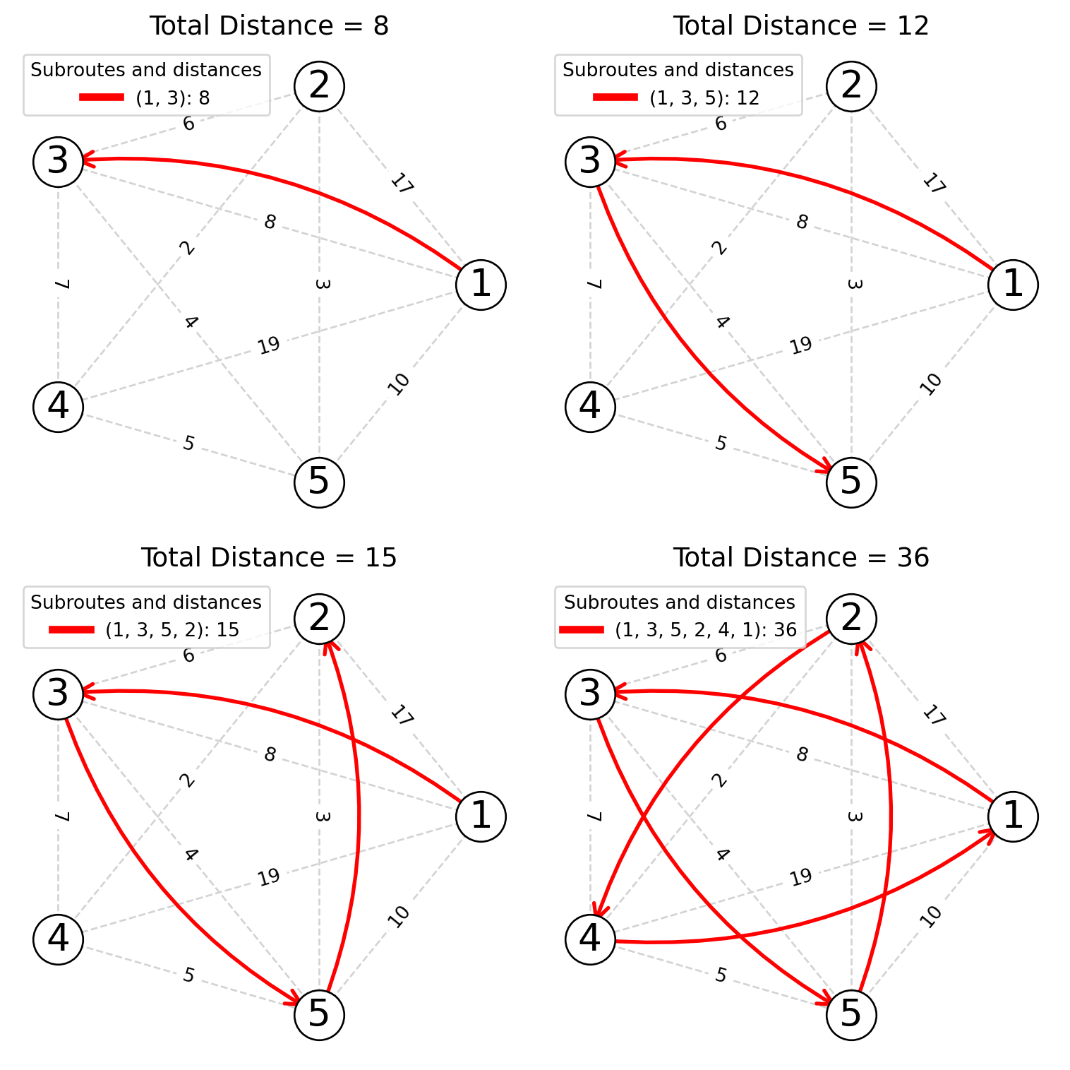
Assuming we start from node 1, we choose the nearest unvisited node at each step until all nodes are visited and then return to the starting node.
| Current Node | Next Node | Distance to Next Node | Cumulative Distance | |
|---|---|---|---|---|
| Step | ||||
| 1 | 1 | 3 | 8 | 8 |
| 2 | 3 | 5 | 4 | 12 |
| 3 | 5 | 2 | 3 | 15 |
| 4 | 2 | 4 | 2 | 17 |
| 5 | 4 | 1 | 19 | 36 |
The route constructed is 1 → 3 → 5 → 2 → 4 → 1 with a total distance of 36.
Clarke-Wright Savings Algorithm
The Clarke-Wright Savings algorithm aims to minimize the total route cost by creating a set of routes that all vehicles will follow, starting and ending at the depot, while serving all demand points exactly once.
Step 1: Calculate the Savings
The algorithm starts by calculating the savings for each pair of demand points \((i, j)\), which is computed using the formula \(S_{ij} = d_{1i} + d_{1j} - d_{ij}\). This savings value represents the cost reduced by directly connecting points \(i\) and \(j\), instead of visiting them separately from the depot.
We calculate the savings:
| Pair \((i,j)\) | \(d_{1i} + d_{1j}\) | \(d_{ij}\) | Savings \(S_{ij}\) |
|---|---|---|---|
| (2, 4) | 17 + 19 = 36 | 2 | 34 |
| (2, 3) | 17 + 8 = 25 | 6 | 19 |
| (2, 5) | 17 + 10 = 27 | 3 | 24 |
| (3, 4) | 8 + 19 = 27 | 7 | 20 |
| (3, 5) | 8 + 10 = 18 | 4 | 14 |
| (4, 5) | 19 + 10 = 29 | 5 | 24 |
Step 2: Rank the Savings
Once all the savings are calculated, they are sorted in descending order. The idea is to prioritize the connections that result in the highest savings, which theoretically contribute most to reducing the overall route cost.
| Pair \((i,j)\) | \(d_{1i} + d_{1j}\) | \(d_{ij}\) | Savings \(S_{ij}\) |
|---|---|---|---|
| (2, 4) | 17 + 19 = 36 | 2 | 34 |
| (2, 5) | 17 + 10 = 27 | 3 | 24 |
| (4, 5) | 19 + 10 = 29 | 5 | 24 |
| (3, 4) | 8 + 19 = 27 | 7 | 20 |
| (2, 3) | 17 + 8 = 25 | 6 | 19 |
| (3, 5) | 8 + 10 = 18 | 4 | 14 |
Warning
Notice that pairs (2,5) and (4,5) have the same savings. The order we choose to break this tie will affect the final route.
Step 3: Build the Routes
This step is where the routes are actually constructed based on the ranked savings list. The algorithm iteratively considers each pair \((i, j)\) from the sorted savings list and decides whether to add the direct link between \(i\) and \(j\) to the current route configuration. The inclusion is based on the following conditions:
- If neither \(i\) nor \(j\) is already included in a route, a new route is initiated.
- If exactly one of the points (\(i\) or \(j\)) is already included in a route and is not an interior point (not sandwiched between two other points not considering the depot), then the link \((i, j)\) is added to that route.
- If both \(i\) and \(j\) are included in different routes and neither is an interior point of its route, the routes are merged.
Repeat Step 3 until all entries have been processed. When the list is fully exhausted, the routes formed constitute the solution to the VRP. Any demand points not included in these routes must be visited individually, starting and ending at the depot.
Breaking Ties in Clarke-Wright
In the Clarke-Wright algorithm, when two pairs have the same savings, the order in which they are considered can affect the final route. Let’s explore two scenarios to illustrate this point.
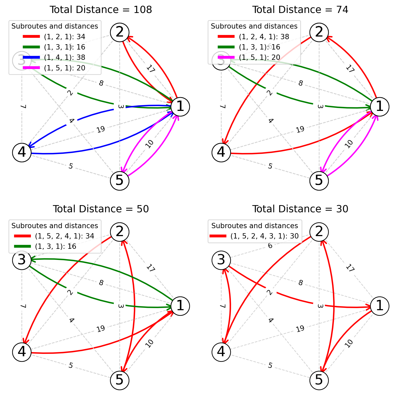
Scenario 1: Choosing (2, 5) Before (4, 5)
This scenario is considered to explore how prioritizing the tie between (2, 5) and (4, 5) in favor of (2, 5) influences the final route.
| Step | Segment Inserted | Resulting Route | Explanation | Arcs Replaced | Cumulative Distance |
|---|---|---|---|---|---|
| 1 | (2, 4) | 1 - 2 - 4 - 1 | Initiating route with highest savings. | (1-2) & (4-1) to (1-2-4) | (17+2+19) |
| 2 | (2, 5) | 1 - 5 - 2 - 4 - 1 | Add link (2-5). | (1-2) & (5-1) to (1-5-2) | (10+3+2+19) |
| 3 | (4, 5) | 1 - 5 - 2 - 4 - 1 | Skipped as 4 and 5 is already included. | - | - |
| 4 | (3, 4) | 1 - 5 - 2 - 4 - 3 - 1 | Add link (3-4). | (1-4) & (3-1) to (1-3-4) | (10+3+2+7+8) |
Notice that the inclusion conditions were as follows:
- Segment (2, 4): Neither 2 nor 4 were included in a route, so a new route was initiated (the current route configuration was empty).
- Segment (2, 5): 5 is not included in a route, and 2 is not an interior point, so the link (2, 5) was added to the route.
- Segment (4, 5): Both 4 and 5 were already included in the route.
- Segment (3, 4): 3 is not included in a route, and 4 is not an interior point, so the link (3, 4) was added to the route.
The route constructed is 1 → 5 → 2 → 4 → 3 → 1 with a total distance of distance 30.
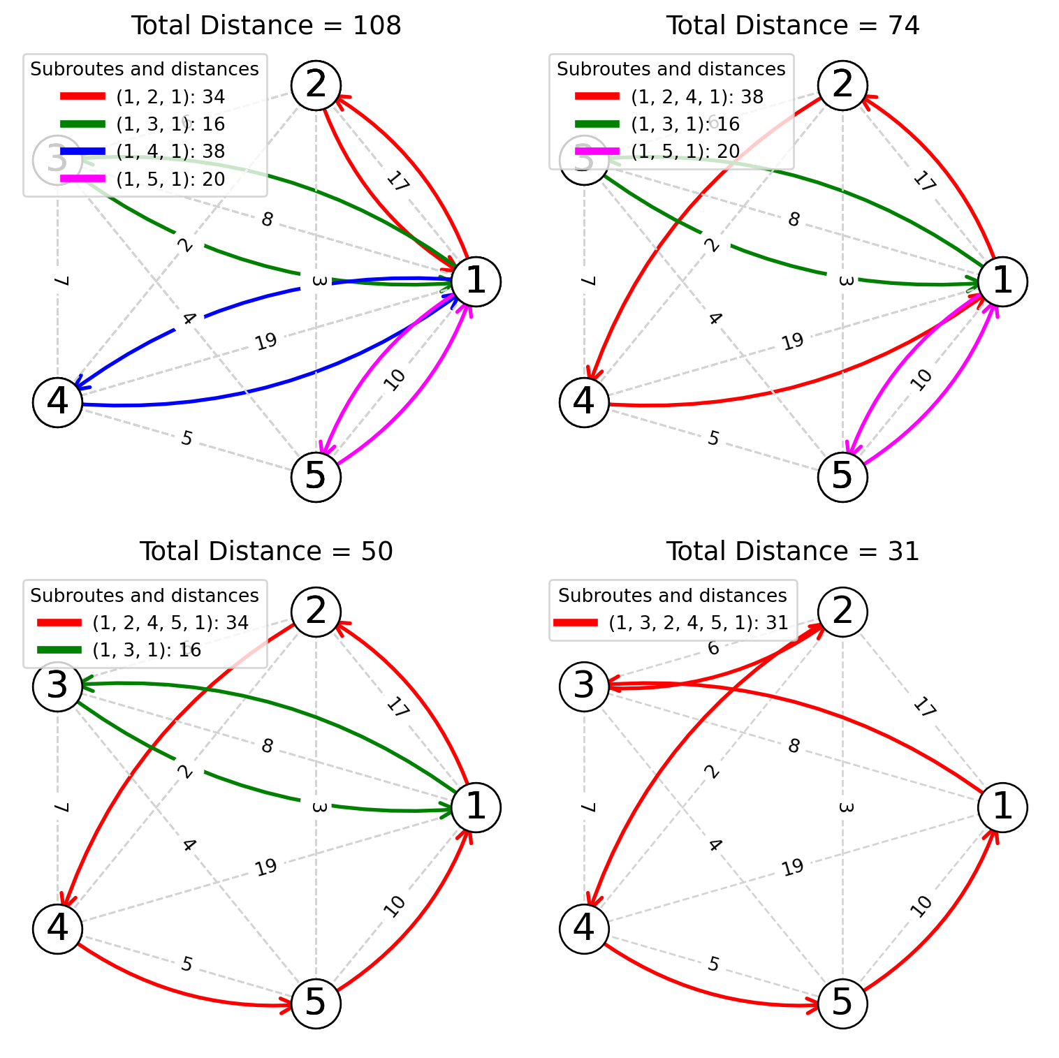
Scenario 2: Choosing (4, 5) Before (2, 5)
This scenario explores the impact of prioritizing the tie between (2, 5) and (4, 5) in favor of (4, 5).
| Step | Segment Inserted | Resulting Route | Explanation | Arcs Replaced | Cumulative Distance |
|---|---|---|---|---|---|
| 1 | (2, 4) | 1 - 2 - 4 - 1 | Initiating route with highest savings. | (1-2) & (4-1) to (1-2-4) | (17+2+19) |
| 2 | (4, 5) | 1 - 2 - 4 - 5 - 1 | Add link (4-5). | (1-4) & (5-1) to (1-5-4) | (17+2+5+10) |
| 3 | (2, 5) | 1 - 2 - 4 - 5 - 1 | Skipped as 2 and 4 already included. | - | - |
| 4 | (3, 4) | 1 - 2 - 4 - 5 - 1 | Skipped as 4 is internal to the route. | - | - |
| 5 | (2, 3) | 1 - 3 - 2 - 4 - 5 - 1 | Add link (3-2). | (1-3) & (2-1) to (1-3-2) | (8+6+2+5+10) |
The route constructed is 1 → 3 → 2 → 4 → 5 → 1 with a total distance of 31 (one unit more than the previous scenario).
Question 2
Capacitated Nearest Neighbor vs. Clarke-Wright. Define and apply a Nearest Neighbor and Clarke-Wright heuristic to find a route for a capacitated vehicle routing problem. The customers are served by the vehicles until the capacity is full. Consider two cases: capacity 200 and 100.
| 0 | 1 | 2 | 3 | 4 | 5 | 6 | 7 | 8 | |
|---|---|---|---|---|---|---|---|---|---|
| 0 | 0 | 26 | 15 | 20 | 7 | 25 | 16 | 24 | 29 |
| 1 | 26 | 0 | 15 | 23 | 26 | 33 | 40 | 38 | 54 |
| 2 | 15 | 15 | 0 | 24 | 13 | 20 | 27 | 35 | 43 |
| 3 | 20 | 23 | 24 | 0 | 26 | 42 | 34 | 15 | 39 |
| 4 | 7 | 26 | 13 | 26 | 0 | 18 | 14 | 31 | 32 |
| 5 | 25 | 33 | 20 | 42 | 18 | 0 | 25 | 49 | 45 |
| 6 | 16 | 40 | 27 | 34 | 14 | 25 | 0 | 32 | 20 |
| 7 | 24 | 38 | 35 | 15 | 31 | 49 | 32 | 0 | 30 |
| Demand | |
|---|---|
| Customer | |
| 1 | 18 |
| 2 | 26 |
| 3 | 11 |
| 4 | 30 |
| 5 | 21 |
| 6 | 16 |
| 7 | 29 |
| 8 | 37 |
Solution Tools
Notice that this question is best solved using tools such Excel or a programming language like Python. The distance matrix is too large to be solved by hand. During exams, you can expect smaller matrices.
Question 2 - Answer
New Rules for Capacitated Case
- If the link to be added properly connects an existing route and the capacity of that route (vehicle) permits so, if not avoid that link.
- If a link is to be added consider two nodes not existing in the current solution, add a new route counting the current weight of that route.
- Two routes can be connected by a feasible link if the capacity of both allows so.
Clarke-Wright Algorithm
Step 1: Calculate the Savings
We use the formula \(s(i, j) = d(0, i) + d(0, j) - d(i, j)\) for every pair \((i, j)\), where \(d(0, i)\) and \(d(0, j)\) are the distances from the depot to points \(i\) and \(j\), respectively, and \(d(i, j)\) is the distance between \(i\) and \(j\).
| Savings | i | j | d(0, i) | d(0, j) | d(i, j) | Result | |
|---|---|---|---|---|---|---|---|
| 0 | (1,2) | 1 | 2 | 26 | 15 | 15 | 26 |
| 1 | (1,3) | 1 | 3 | 26 | 20 | 23 | 23 |
| 2 | (1,4) | 1 | 4 | 26 | 7 | 26 | 7 |
| 3 | (1,5) | 1 | 5 | 26 | 25 | 33 | 18 |
| 4 | (1,6) | 1 | 6 | 26 | 16 | 40 | 2 |
| 5 | (1,7) | 1 | 7 | 26 | 24 | 38 | 12 |
| 6 | (1,8) | 1 | 8 | 26 | 29 | 54 | 1 |
| 7 | (2,3) | 2 | 3 | 15 | 20 | 24 | 11 |
| 8 | (2,4) | 2 | 4 | 15 | 7 | 13 | 9 |
| 9 | (2,5) | 2 | 5 | 15 | 25 | 20 | 20 |
| 10 | (2,6) | 2 | 6 | 15 | 16 | 27 | 4 |
| 11 | (2,7) | 2 | 7 | 15 | 24 | 35 | 4 |
| 12 | (2,8) | 2 | 8 | 15 | 29 | 43 | 1 |
| 13 | (3,4) | 3 | 4 | 20 | 7 | 26 | 1 |
| 14 | (3,5) | 3 | 5 | 20 | 25 | 42 | 3 |
| 15 | (3,6) | 3 | 6 | 20 | 16 | 34 | 2 |
| 16 | (3,7) | 3 | 7 | 20 | 24 | 15 | 29 |
| 17 | (3,8) | 3 | 8 | 20 | 29 | 39 | 10 |
| 18 | (4,5) | 4 | 5 | 7 | 25 | 18 | 14 |
| 19 | (4,6) | 4 | 6 | 7 | 16 | 14 | 9 |
| 20 | (4,7) | 4 | 7 | 7 | 24 | 31 | 0 |
| 21 | (4,8) | 4 | 8 | 7 | 29 | 32 | 4 |
| 22 | (5,6) | 5 | 6 | 25 | 16 | 25 | 16 |
| 23 | (5,7) | 5 | 7 | 25 | 24 | 49 | 0 |
| 24 | (5,8) | 5 | 8 | 25 | 29 | 45 | 9 |
| 25 | (6,7) | 6 | 7 | 16 | 24 | 32 | 8 |
| 26 | (6,8) | 6 | 8 | 16 | 29 | 20 | 25 |
| 27 | (7,8) | 7 | 8 | 24 | 29 | 30 | 23 |
Step 2: Rank the Savings
Sort the savings in descending order to prioritize the pairs with the highest savings, as they are the most beneficial in reducing the total route distance.
| Savings | i | j | d(0, i) | d(0, j) | d(i, j) | Result | |
|---|---|---|---|---|---|---|---|
| 0 | (3,7) | 3 | 7 | 20 | 24 | 15 | 29 |
| 1 | (1,2) | 1 | 2 | 26 | 15 | 15 | 26 |
| 2 | (6,8) | 6 | 8 | 16 | 29 | 20 | 25 |
| 3 | (1,3) | 1 | 3 | 26 | 20 | 23 | 23 |
| 4 | (7,8) | 7 | 8 | 24 | 29 | 30 | 23 |
| 5 | (2,5) | 2 | 5 | 15 | 25 | 20 | 20 |
| 6 | (1,5) | 1 | 5 | 26 | 25 | 33 | 18 |
| 7 | (5,6) | 5 | 6 | 25 | 16 | 25 | 16 |
| 8 | (4,5) | 4 | 5 | 7 | 25 | 18 | 14 |
| 9 | (1,7) | 1 | 7 | 26 | 24 | 38 | 12 |
| 10 | (2,3) | 2 | 3 | 15 | 20 | 24 | 11 |
| 11 | (3,8) | 3 | 8 | 20 | 29 | 39 | 10 |
| 12 | (5,8) | 5 | 8 | 25 | 29 | 45 | 9 |
| 13 | (2,4) | 2 | 4 | 15 | 7 | 13 | 9 |
| 14 | (4,6) | 4 | 6 | 7 | 16 | 14 | 9 |
| 15 | (6,7) | 6 | 7 | 16 | 24 | 32 | 8 |
| 16 | (1,4) | 1 | 4 | 26 | 7 | 26 | 7 |
| 17 | (4,8) | 4 | 8 | 7 | 29 | 32 | 4 |
| 18 | (2,7) | 2 | 7 | 15 | 24 | 35 | 4 |
| 19 | (2,6) | 2 | 6 | 15 | 16 | 27 | 4 |
| 20 | (3,5) | 3 | 5 | 20 | 25 | 42 | 3 |
| 21 | (1,6) | 1 | 6 | 26 | 16 | 40 | 2 |
| 22 | (3,6) | 3 | 6 | 20 | 16 | 34 | 2 |
| 23 | (1,8) | 1 | 8 | 26 | 29 | 54 | 1 |
| 24 | (3,4) | 3 | 4 | 20 | 7 | 26 | 1 |
| 25 | (2,8) | 2 | 8 | 15 | 29 | 43 | 1 |
| 26 | (5,7) | 5 | 7 | 25 | 24 | 49 | 0 |
| 27 | (4,7) | 4 | 7 | 7 | 24 | 31 | 0 |
Notice that are some ties:
| Savings | i | j | d(0, i) | d(0, j) | d(i, j) | Result | |
|---|---|---|---|---|---|---|---|
| 3 | (1,3) | 1 | 3 | 26 | 20 | 23 | 23 |
| 4 | (7,8) | 7 | 8 | 24 | 29 | 30 | 23 |
| 12 | (5,8) | 5 | 8 | 25 | 29 | 45 | 9 |
| 13 | (2,4) | 2 | 4 | 15 | 7 | 13 | 9 |
| 14 | (4,6) | 4 | 6 | 7 | 16 | 14 | 9 |
| 17 | (4,8) | 4 | 8 | 7 | 29 | 32 | 4 |
| 18 | (2,7) | 2 | 7 | 15 | 24 | 35 | 4 |
| 19 | (2,6) | 2 | 6 | 15 | 16 | 27 | 4 |
| 21 | (1,6) | 1 | 6 | 26 | 16 | 40 | 2 |
| 22 | (3,6) | 3 | 6 | 20 | 16 | 34 | 2 |
| 23 | (1,8) | 1 | 8 | 26 | 29 | 54 | 1 |
| 24 | (3,4) | 3 | 4 | 20 | 7 | 26 | 1 |
| 25 | (2,8) | 2 | 8 | 15 | 29 | 43 | 1 |
| 26 | (5,7) | 5 | 7 | 25 | 24 | 49 | 0 |
| 27 | (4,7) | 4 | 7 | 7 | 24 | 31 | 0 |
Step 3: Build the Routes
Vehicle Capacity = 200
- At first tie, use \(s(1,3)\) before \(s(7,8)\)
- Routes:
- 0 → 3 → 7 → 0
- 0 → 1 → 2 → 0
- 0 → 6 → 8 → 0
- Final route after applying \(s(1,3)\): 0 → 2 → 1 → 3 → 7 → 8 → 6 → 0
- Cost = 164
- Routes:
- Now, at first tie use \(s(7,8)\) before \(s(1,3)\)
- Routes:
- 0 → 3 → 7 → 0
- 0 → 1 → 2 → 0
- 0 → 6 → 8 → 0
- Final route after applying \(s(7,8)\): 0 → 6 → 8 → 7 → 3 → 1 → 2 → 0
- Cost remains the same.
- Routes:
Vehicle Capacity = 100
- At first tie, use \(s(1,3)\) before \(s(7,8)\)
- Initial routes:
- 0 → 3 → 7 → 0
- 0 → 1 → 2 → 0
- 0 → 6 → 8 → 0
- Adjusted routes for capacity constraints:
- 0 → 2 → 1 → 3 → 7 → 0
- 0 → 5 → 6 → 8 → 0
- 0 → 4 → 0
- Total Cost = 205
- Initial routes:
- Now, at first tie use \(s(7,8)\) before \(s(1,3)\)
- Initial routes:
- 0 → 3 → 7 → 0
- 0 → 1 → 2 → 0
- 0 → 6 → 8 → 0
- Adjusted routes for capacity constraints:
- 0 → 3 → 7 → 8 → 6 → 0
- 0 → 1 → 2 → 5 → 4 → 0
- Total Cost = 187
- Initial routes:
This solution with two routes (187 versus 205) is better than the solution above.
Question 3
Construction Heuristics Truck Loading. Given the set of items in Table 9 with specific weights, volumes, and values, your task is to select a subset of these items to maximize the total value while adhering to the weight and volume constraints of the truck. The truck can carry a maximum weight of 10 units and a maximum volume of 20 units.
| Item | Value | Weight | Volume |
|---|---|---|---|
| 1 | 4 | 3 | 5 |
| 2 | 6 | 5 | 8 |
| 3 | 3 | 4 | 7 |
| 4 | 5 | 2 | 3 |
- Formulate the problem indicating the objective, decision variables, and constraints.
- Design and describe a constructive algorithm for this problem using a pseudocode or flowchart.
- Describe the steps of the algorithm using the toy example provided in the table above.
Question 3 - Answer
1. Mathematical Model
Indices:
- Let \(i\) be the index used to refer to items, where \(i = 1, 2, ..., n\).
Sets:
- Let \(N\) be the set of all items, where \(N = \{1, 2, ..., n\}\).
Parameters:
- \(v_i\): Value of item \(i\), representing the benefit or profit of selecting item \(i\).
- \(w_i\): Weight of item \(i\), indicating how heavy the item is.
- \(vol_i\): Volume of item \(i\), indicating how much space the item occupies.
- \(mW\): Maximum allowable weight, the weight capacity of the truck.
- \(mV\): Maximum allowable volume, the volume capacity of the truck.
Decision Variables:
- \(x_i\): Binary decision variable where \(x_i = 1\) if item \(i\) is selected (loaded into the truck) and \(0\) otherwise.
Objective Function:
Maximize the total value of the items selected to be loaded into the truck:
\[\text{Maximize } Z = \sum_{i \in N} x_i \cdot v_i\]
Constraints:
Weight Constraint: Ensures that the total weight of the selected items does not exceed the truck’s weight capacity.
\[\sum_{i \in N} x_i \cdot w_i \leq mW\]
Volume Constraint: Ensures that the total volume of the selected items does not exceed the truck’s volume capacity.
\[\sum_{i \in N} x_i \cdot vol_i \leq mV\]
Binary Constraints: Ensures that each item is either selected or not selected, with no partial selection allowed.
\[x_i \in \{0, 1\} \text{ for all } i \in N\]
2. Constructive Algorithm
Input: Set \(N\), values \(v_i\), totalWeight \(w_i\), volumes \(vol_i\), maximum weight \(mW\), maximum volume \(mV\)
Output: Set \(S\) representing the selected items
Variables:
- \(S\): A set to store the indices of items selected to maximize the total value while adhering to weight and volume constraints.
- \(totalValue\): The total value of the items in the set \(S\).
- \(totalWeight\): The total weight of the items in the set \(S\).
- \(totalVolume\): The total volume of the items in the set \(S\).
- \(i\): Index variable used to iterate through the items.
Procedure:
- Initialize \(S = \emptyset\) (an empty set), \(totalValue = 0\) (initial total value), \(totalWeight = 0\) (initial total weight), \(totalVolume = 0\) (initial total volume).
- For each item \(i\) in the set \(N\) do:
- 2.1. If adding item \(i\) does not exceed the maximum weight \(mW\) and volume \(mV\) constraints:
- 2.1.1. Add item \(i\) to the set \(S\).
- 2.1.2. Update \(totalValue\) to include the value of item \(i\): \(totalValue = totalValue + v_i\).
- 2.1.3. Update the total weight of the set \(S\): \(totalWeight = totalWeight + w_i\).
- 2.1.4. Update the total volume of the set \(S\): \(totalVolume = totalVolume + vol_i\).
- 2.1. If adding item \(i\) does not exceed the maximum weight \(mW\) and volume \(mV\) constraints:
- Return the set \(S\) as the solution, containing the indices of the items that maximize the total value without exceeding the capacity constraints.
flowchart TD
    A(("Start")) --> B[/"N (set of items i)<br>v_i (item profit),<br>w_i (item weight),<br>vol_i (item volume),<br>mW (max. weight),<br>mV (max. volume)"/]
    B --> C["Initialize:<br>S = ∅ (Set of selected items),<br>totalValue = 0,<br>totalWeight = 0,<br>totalVolume = 0"]
    C --> D["For each item i in N"]
    D --> E{"totalWeight + w_i ≤ mW <br> AND <br> totalVolume + vol_i ≤ mV"}
    E -- "Yes" --> F["Add item i to S"]
    F --> G["totalValue = totalValue + v_i <br> totalWeight = totalWeight + w_i <br> totalVolume = totalVolume + vol_i"]
    G --> H{"More items in N?"}
    E -- "No" --> H
    H -- "Yes" --> D
    H -- "No" --> I[/S/]
    I --> J(("End"))
Toy Example
Input Data:
Truck’s maximum weight capacity (\(mW\)): 10 units
Truck’s maximum volume capacity (\(mV\)): 20 units
Items details:
Table 10: Data for the items to be loaded into the truck. Item (\(i\)) Value (\(v_i\)) Weight (\(w_i\)) Volume (\(vol_i\)) 1 4 3 5 2 6 5 8 3 3 4 7 4 5 2 3
Construction Heuristics Steps:
| Step | Item Considered | Action | Set \(S\) | totalValue |
totalWeight |
totalVolume |
|---|---|---|---|---|---|---|
| 1 | - | Initialize | \(\{\}\) | 0 | 0 | 0 |
| 2 | 1 | Add | \(\{1\}\) | 4 | 3 | 5 |
| 3 | 2 | Add | \(\{1, 2\}\) | 10 | 8 | 13 |
| 4 | 3 | Skip | \(\{1, 2\}\) | 10 | 8 | 13 |
| 5 | 4 | Add | \(\{1, 2, 4\}\) | 15 | 10 | 16 |
Explanation:
- Step 1: Initialize the algorithm with an empty set \(S\), and zero values for
totalValue,totalWeight, andtotalVolume. - Step 2: Item 1 fits within the constraints, so it’s added to the set \(S\).
totalValue,totalWeight, andtotalVolumeare updated accordingly. - Step 3: Item 2 also fits, so it’s added. The cumulative values are updated.
- Step 4: Item 3 is skipped as adding it would exceed the maximum weight capacity.
- Step 5: Item 4 is added since it fits within the remaining capacity, and all cumulative values are updated.
The final selection of items is \(\{1, 2, 4\}\), with a total value (totalValue) of 15, a total weight (totalWeight) of 10, and a total volume (totalVolume) of 16.
Question 4
Local Search. Given the distance matrix (\(d_{ij}\)) presented in Table 11, describe and apply the Nearest Neighbor and Clarke-Wright heuristics to determine a route. The depot is located at node 1, and only one vehicle is available.
| 1 | 2 | 3 | 4 | |
|---|---|---|---|---|
| Node ID | ||||
| 1 | 0 | 17 | 8 | 19 |
| 2 | 17 | 0 | 6 | 2 |
| 3 | 8 | 6 | 0 | 7 |
| 4 | 19 | 2 | 7 | 0 |
Next, devise and implement a local search starting from both your Nearest Neighbor and Clarke-Wright solutions.
Question 4 - Answer
Hint: After applying the Clarke-Wright and the Nearest Neighbor heuristics, you could define the neighborhood as follows:
- N: Set of customers.
- s: A solution to the problem, e.g., s = (1,2,3,4), representing the route 1 → 2 → 3 → 4 → 1.
The swap neighborhood is defined as:
\[ N_{\text{swap}}(s) = \{ (i, j) \in N \mid i \neq j, \text{ interchange } i \text{ and } j \text{ in } s \} \]
For the solution s = (1,2,3,4), its neighborhood is:
- (2,1,3,4) - swap 1 and 2
- (3,2,1,4) - swap 1 and 3
- (4,2,3,1) - swap 1 and 4
- (1,3,2,4) - swap 2 and 3
- (1,4,3,2) - swap 2 and 4
- (1,2,4,3) - swap 3 and 4
where each element is a variation of s obtained by swapping two nodes.
Note that fully solving the problem entails:
- Defining the neighborhood.
- Providing a detailed description of the local search algorithm.
- Applying the local search algorithm to the initial solutions obtained by the Clarke-Wright and Nearest Neighbor heuristics, demonstrating the iterations and the final solution.
Next, you can compare which construction heuristic (Clarke-Wright or Nearest Neighbor) provides a better initial solution for the local search algorithm.
Question 5
Enhanced Clark and Wright. Consider the enhanced Clark and Wright method proposed in:
Altınel, İ. K., & Öncan, T. (2005). A new enhancement of the Clarke and Wright savings heuristic for the capacitated vehicle routing problem. Journal of the Operational research Society, 56(8), 954-961.
Apply this method to refuse collection problem described here. For simplicity, consider only 5 customers (2-6) and a capacity of 12.
Compare to the standard Clarke and Wright solution. Which is better? Select the parameters that you consider convenient after checking the paper.
Question 5 - Answer
Hint: As the first step, you can use previous information removing nodes from 7 to 10. Then you obtain the Clarke and Wright solution. For the Altinel and Oncan method, it is just applying the formula provided by them and calculate the new savings. Checking the paper, you can see that they use different parameter configurations. You can select the ones that you think provided the best results.
Question 6
Clarke and Wright with Time Windows. How to adapt Clarke and Wright for working with time windows?
Question 6 - Answer
Hint: You have to consider now all possible directions. It is not the same, in terms of time windows feasibility, visiting customer in order \((i,j)\) and \((j,i)\).
Question 7
Giant Tour. Given the following giant tour, optimally split it. The demand of the customers (i.e., a, b, c, d, e) is given in parentheses. You have at most 4 vehicles. Analyze the case with and without capacity restriction of 10 associated with the vehicles.
Question 7 - Answer
Prins, Lacomme, and Prodhon (2014) proposes two algorithms (viz., Split and Extract), but also mentions a classical method to solve the CVRP using an auxiliary graph \(H=(Y,U)\) and then using the Bellman algorithm to find the shortest path. In the following we will describe the classical method to solve the CVRP using an auxiliary graph \(H=(Y,U)\) and then using the Bellman algorithm to find the shortest path.
You are encouraged to read the paper and apply the faster algorithms (Split and Extract) to the same problem and check if the results match.
Problem Definition
Table 12 shows the key notation used in the algorithms.
| Symbol | Definition |
|---|---|
| \(n\) | Number of customers. |
| \(T=(T_1,\dots,T_n)\) | Ordered list of customers to be served in that sequence (the giant tour). |
| \(q(T_i)\) | Demand of customer \(T_i\). |
| \(Q\) | Vehicle capacity. A sub‐route \((T_i,\dots,T_j)\) is feasible if \(\sum_{k=i}^j q(T_k) \le Q\). |
| \(s(T_i)\) | Service time at customer \(T_i\). |
| \(c(u,v)\) | Travel cost from node \(u\) to node \(v\). |
| \(\text{cost}(i,j)\) | Cost of a sub‐route serving customers \((T_i,\dots,T_j)\), including departure from the depot, service times, travel between customers, and return to the depot. Formally: \(\displaystyle \text{cost}(i,j) \;=\; c(0,T_i)\;+\;\sum_{k=i}^{j-1}\Bigl[s(T_k) + c(T_k,T_{k+1})\Bigr]\;+\;s(T_j)\;+\;c(T_j,0)\). |
| \(V_j\) | Minimal cost to serve the first \(j\) customers \((T_1,\dots,T_j)\) under the given order. |
| \(Y = \{0,1,\dots,n\}\) | Node set of the auxiliary graph. Node \(j\) represents “customers up to \(T_j\) have been served.” Node \(0\) is the “start” (no customers served yet). |
| \((i-1 \to j)\) | Arc from node \((i-1)\) to node \(j\) if the subsequence \((T_i,\dots,T_j)\) fits in one vehicle trip. This arc is weighted by \(\text{cost}(i,j)\). |
| \(U\) | Arc set of the auxiliary graph. Each feasible subsequence \((T_i,\dots,T_j)\) with \(\sum_{k=i}^j q(T_k) \le Q\) corresponds to an arc \((i-1 \to j)\) in \(H\). |
Using the elements from Table 12, we can define the problem:
- Customers:
- Number of customers: \(n=5\).
- Ordered list of customers: \(T=(a,b,c,d,e)\).
- Demands: \(q(a)=5\), \(q(b)=4\), \(q(c)=4\), \(q(d)=2\), \(q(e)=7\)
- Service times: \(s(\cdot)=0\)
- Vehicle: Capacity \(Q=10\).
- Travel Costs:
- \(c(0,a)=20\), \(c(0,b)=25\), \(c(0,c)=30\), \(c(0,d)=40\), \(c(0,e)=35\).
- \(c(a,b)=10\), \(c(b,c)=30\), \(c(c,d)=25\), \(c(d,e)=15\).
- Sub‐route Costs: The subroute costs to serve customers \((T_i,\dots,T_j)\):
- \(\text{cost}(a) = 40\) (demand 5).
- \(\text{cost}(a,b) = 55\) (demand 9).
- \(\text{cost}(a,b,c) = 85\) (demand 13).
- \(\text{cost}(a,b,c,d) = 120\) (demand 15).
- … (note that some subsequences are infeasible due to demand exceeding \(Q\)).
Building the Auxiliary Graph \((Y,U)\)
In the auxiliary graph \(H=(Y,U)\), the nodes \(Y = \{0,1,2,3,4,5\}\) correspond to having served up to customer \(T_j\) (with \(j=0\) meaning no customers served yet). For each subsequence \((T_i,\dots,T_j)\) that fits in one vehicle trip (\(\sum_{k=i}^j q(T_k)\le Q\)), we create an arc \((i-1 \to j)\) with weight \(\text{cost}(i,j)\). An arc \((i-1 \to j)\) corresponds to a feasible sub‐route \((T_i,\dots,T_j)\) with total demand \(\le Q\). For example, \((0\to1)\) corresponds to serving customer \(a\) whereas \((0\to2)\) corresponds to serving customers \((a,b)\).
Table 13 shows all possible \((i,j)\) pairs, along with the load, feasibility, and arc cost. Infesible arcs consist of subsequences with total demand exceeding the vehicle capacity \(Q=10\).
| \(\mathbf{i}\) | \(\mathbf{j}\) | Subsequence \((T_i,\dots,T_j)\) | Load \(\sum_{k=i}^j q(T_k)\) | Feasible? (\(\le Q=10\)) | Arc \((i-1 \to j)\)? | \(\text{cost}(i,j)\) | Explanation |
|---|---|---|---|---|---|---|---|
| 1 | 1 | \((a)\) | \(5\) | Yes | \((0 \to 1)\) | 40 | Single trip \((a)\) => 40. |
| 1 | 2 | \((a,b)\) | \(9\) | Yes | \((0 \to 2)\) | 55 | Sub‐route \((a,b)\) => 55. |
| 1 | 3 | \((a,b,c)\) | \(13\) | No | — | — | Load 13 > 10 => infeasible. |
| 1 | 4 | \((a,b,c,d)\) | \(15\) | No | — | — | Load 15 > 10 => infeasible. |
| 1 | 5 | \((a,b,c,d,e)\) | \(22\) | No | — | — | Load 22 > 10 => infeasible. |
| 2 | 2 | \((b)\) | \(4\) | Yes | \((1 \to 2)\) | 50 | Single trip \((b)\) => 50. |
| 2 | 3 | \((b,c)\) | \(8\) | Yes | \((1 \to 3)\) | 85 | Sub‐route \((b,c)\) => 85. |
| 2 | 4 | \((b,c,d)\) | \(10\) | Yes | \((1 \to 4)\) | 120 | Sub‐route \((b,c,d)\) => 120. |
| 2 | 5 | \((b,c,d,e)\) | \(17\) | No | — | — | Load 17 > 10 => infeasible. |
| 3 | 3 | \((c)\) | \(4\) | Yes | \((2 \to 3)\) | 60 | Single trip \((c)\) => 60. |
| 3 | 4 | \((c,d)\) | \(6\) | Yes | \((2 \to 4)\) | 95 | Sub‐route \((c,d)\) => 95. |
| 3 | 5 | \((c,d,e)\) | \(13\) | No | — | — | Load 13 > 10 => infeasible. |
| 4 | 4 | \((d)\) | \(2\) | Yes | \((3 \to 4)\) | 80 | Single trip \((d)\) => 80. |
| 4 | 5 | \((d,e)\) | \(9\) | Yes | \((3 \to 5)\) | 90 | Sub‐route \((d,e)\) => 90. |
| 5 | 5 | \((e)\) | \(7\) | Yes | \((4 \to 5)\) | 70 | Single trip \((e)\) => 70. |
Thus, the feasible arcs \(U\) in \(H\) are:
- \(0\to1\) (cost 40), \(0\to2\) (cost 55)
- \(1\to2\) (50), \(1\to3\) (85), \(1\to4\) (120)
- \(2\to3\) (60), \(2\to4\) (95)
- \(3\to4\) (80), \(3\to5\) (90)
- \(4\to5\) (70)
Shortest‐Path (Bellman) in Topological Order
Because \(H\) is a directed acyclic graph (DAG) with edges from lower to higher node indices, we can do a Bellman* (or dynamic programming) pass from left to right. We keep a label \(V_j\) for each node \(j\), initialized to \(\infty\) except \(V_0=0\). Each time we relax an edge \((i\to j)\), we check if \(V_i + \text{cost}(i\to j)\) improves \(V_j\).
Table 14 shows the Bellman pass to find the minimal cost to serve all customers in the given order.
| Iteration | Node Processed | Relaxed Arcs & Updates | \(V_0\) | \(V_1\) | \(V_2\) | \(V_3\) | \(V_4\) | \(V_5\) |
|---|---|---|---|---|---|---|---|---|
| Init | — | \(V_0=0\), \(V_1=V_2=V_3=V_4=V_5=\infty\) | 0 | \(\infty\) | \(\infty\) | \(\infty\) | \(\infty\) | \(\infty\) |
| 1 | 0 | - Relax \((0\to1)\): \(V_1=\min(\infty, 0+40)=40\) - Relax \((0\to2)\): \(V_2=55\) |
0 | 40 | 55 | \(\infty\) | \(\infty\) | \(\infty\) |
| 2 | 1 | - Relax \((1\to2)\): new cost= \(40+50=90\), but \(V_2=55\) better, no update - Relax \((1\to3)\): \(V_3=\min(\infty, 40+85)=125\) - Relax \((1\to4)\): \(V_4=40+120=160\) |
0 | 40 | 55 | 125 | 160 | \(\infty\) |
| 3 | 2 | - Relax \((2\to3)\): new cost= \(55+60=115\), improves old \(125\), so \(V_3=115\) - Relax \((2\to4)\): new cost= \(55+95=150\), improves old \(160\), so \(V_4=150\) |
0 | 40 | 55 | 115 | 150 | \(\infty\) |
| 4 | 3 | - Relax \((3\to4)\): new cost= \(115+80=195\), worse than \(150\), no update - Relax \((3\to5)\): \(V_5=\min(\infty,115+90)=205\) |
0 | 40 | 55 | 115 | 150 | 205 |
| 5 | 4 | - Relax \((4\to5)\): new cost= \(150+70=220\), worse than \(205\), no update | 0 | 40 | 55 | 115 | 150 | 205 |
| 6 | 5 | - No outgoing arcs from node 5. Done. | 0 | 40 | 55 | 115 | 150 | 205 |
At the end, \(V_5=205\) is the minimal cost to serve all 5 customers in the given order. The path that yields \(205\) is \(0\to2\to3\to5\), corresponding to three sub‐routes:
- \((a,b)\) from node 0 to node 2 (cost 55),
- \((c)\) from node 2 to node 3 (cost 60),
- \((d,e)\) from node 3 to node 5 (cost 90).
Summing up \(55 + 60 + 90 = 205\). The shortest path is shown in Figure 6. Notice that each path corresponds to a feasible sub‐route with total demand \(\le Q=10\). Therefore, if
Figure 7 shows the three sub‐routes found in the giant tour.
Question 8
K-Means Algorithm for CVRP. Design a k-means clustering algorithm for the Capacitated Vehicle Routing Problem (CVRP) that accounts for the demand at each point.
Question 8 - Answer
Before solving this exercise, review the k-means algorithm in Section 1.1.
Hint: To account for vehicle capacity, modify the line \[ i = \arg\min_{j=1,\ldots,k} \| p - c_j \|^2 \] by adding a condition that only considers indices \(i\) for which the corresponding cluster has available capacity. Thus, you will need to keep track of the current load for each cluster across iterations.
Question 9
Solomon Nearest Neighbor Insertion. Consider one hour travel time between any two customers (\(d_ij\)). Zero delivery time at each customer (\(s_i=0\)). No distances considered (\(\lambda_1=0\)). Depot is open 24hs. \(\lambda_2=0.5\). How is total sum of traveling time?
Question 9 - Answer
- Create a new metric \(𝑐_{𝑖𝑗}\) to determine closest customer based on:
- \(𝑇_{𝑖𝑗}=𝑏_𝑗−(𝑏_𝑖+𝑠_𝑖)\)
- \(𝑣_{𝑖𝑗}=𝑙_𝑗−(𝑏_𝑖+𝑠_𝑖+𝑡_{𝑖𝑗} )\)
- \(𝑐_{𝑖𝑗}=\lambda_1 𝑑_{𝑖𝑗}+\lambda_2 𝑇_{𝑖𝑗}+\lambda_3 𝑣_{𝑖𝑗}\)
- \(\lambda_1+\lambda_2+\lambda_3=1\)
- Select the customers in a constructive way using \(𝑐_{𝑖𝑗}\).
Notation:
- Customers time Windows: \([𝑒_𝑖,𝑙_𝑖]\).
- Travel time between any two customers (\(𝑡_{𝑖𝑗}\)).
- Distance between any two customers (\(𝑑_{𝑖𝑗}\)).
- Service time at each customer (\(𝑠_𝑖\)).
- \(𝑏_𝑗\), service beginning at node \(j\); \(𝑏_𝑗=\max(𝑒_𝑗,𝑏_𝑖+𝑠_𝑖+𝑡_{𝑖𝑗})\)
Notice that \(\lambda_{1} + \lambda_{2} + \lambda_{3} = 1\), since the distance does not have to be considered for the arcs’ cost, then \(\lambda_{1} = 0\), and since \(\lambda_{2} = 0.5\). Hence, \(\lambda_{3} = 0.5\).
Find a calculation from the depot to the first node, you will have to do it for all nodes. Consider that depot is 0 as time windows is not given.
- \(T_{01}=9-0+0=9\) (beginning of service)
- \(v_{01}=12-(0+1)=11\) (urgency of delivery)
- \(c_{01}= 0.5*9+0.5*11=10\)
You have to perform the same process for all nodes \(n\) and then select the one with the least cost \(c_{0n}\). Afterwards, you need to repeat calculations to from \(n\) to remaining nodes to select the next one. Notice that for node \(n\), \(b_n\) is the time that you set up when you arrived.
References
K-means Clustering
The basic K-means algorithm is as follows:
- Select \(k\) points as initial centroids.
- Repeat:
- Form \(k\) clusters by assigning each point to its closest centroid.
- Recompute the centroid of each cluster.
- Until the centroids do not change.
Using more detailed pseudocode, the K-means algorithm can be described as follows:
Input:
- A point set \(P \subseteq \mathbb{R}^d\)
- Number of centers \(k\)
- Distance function \(d: \mathbb{R}^d \times \mathbb{R}^d \rightarrow \mathbb{R}\)
Output: Centers \(c_1, \ldots, c_k\)
Algorithm:
- Choose initial centers \(c_1, \ldots, c_k\) from \(\mathbb{R}^d\).
- Repeat:
- Set \(P_1, \ldots, P_k \leftarrow \emptyset\).
- For each \(p \in P\) do:
- Compute \(i\), the centroid closest to \(p\), as: \[i = \arg\min_{j=1,\ldots,k} \| p - c_j \|^2.\]
- Update \(P_i \leftarrow P_i \cup \{p\}\).
- For \(i = 1\) to \(k\) do:
- If \(P_i \neq \emptyset\) then update \[ c_i = \frac{1}{|P_i|} \sum_{p \in P_i} p. \]
- Until the centers do not change.
Euclidean Distance in K-means Clustering
The expression \(\|p - c_i\|^2\) represents the square of the Euclidean distance between the point \(p\) and the centroid \(c_i\).
Therefore:
- \(p - c_i\) is the difference vector between the coordinates of \(p\) and \(c_i\) in a \(d\)-dimensional space.
- \(\|p - c_i\|\) calculates the Euclidean distance (or length) of that difference vector.
- \(\|p - c_i\|^2\) gives the sum of the squared differences of their components.
For example, if \(d = 2\), and \(p = (p_1, p_2)\) and \(c_i = (c_{i1}, c_{i2})\), then:
\(\|p - c_i\|^2 = (p_1 - c_{i1})^2 + (p_2 - c_{i2})^2\).
Why use the squared Euclidean distance instead of the standard Euclidean distance?
- Taking the square root is computationally more expensive, especially when you’re just comparing distances.
- Squaring the differences gives more weight to larger differences, which can be useful in some contexts.
How to Interpret the \(\arg\min\) Notation
In the expression
\[ i = \arg\min_{j=1,\ldots,k} \| p - c_j \|^2, \]
the variable \(j\) serves as a dummy variable that iterates over all centroid indices from 1 to \(k\). It is a placeholder that represents each candidate index for the centroids. The \(\arg\min\) notation indicates that we are looking for the value of \(j\) that minimizes the expression \(\| p - c_j \|^2\). This value is then assigned to \(i\), which identifies the centroid \(c_i\) that is closest to the point \(p\).
References
Prins, Christian, Philippe Lacomme, and Caroline Prodhon. 2014. “Order-First Split-Second Methods for Vehicle Routing Problems: A Review.” Transportation Research Part C: Emerging Technologies 40 (March): 179–200. https://doi.org/10.1016/j.trc.2014.01.011.