| D1 | D2 | S1 | S2 | S3 | |
|---|---|---|---|---|---|
| P1 | 8.0 | 14.0 | inf | inf | inf |
| P2 | 12.0 | 10.0 | inf | inf | inf |
| P3 | 16.0 | 12.0 | inf | inf | inf |
| D1 | inf | inf | 10.0 | 8.0 | 12.0 |
| D2 | inf | inf | 6.0 | 15.0 | 9.0 |
Practice Exam (Solutions)
Scenario 1 - Brewery Distribution
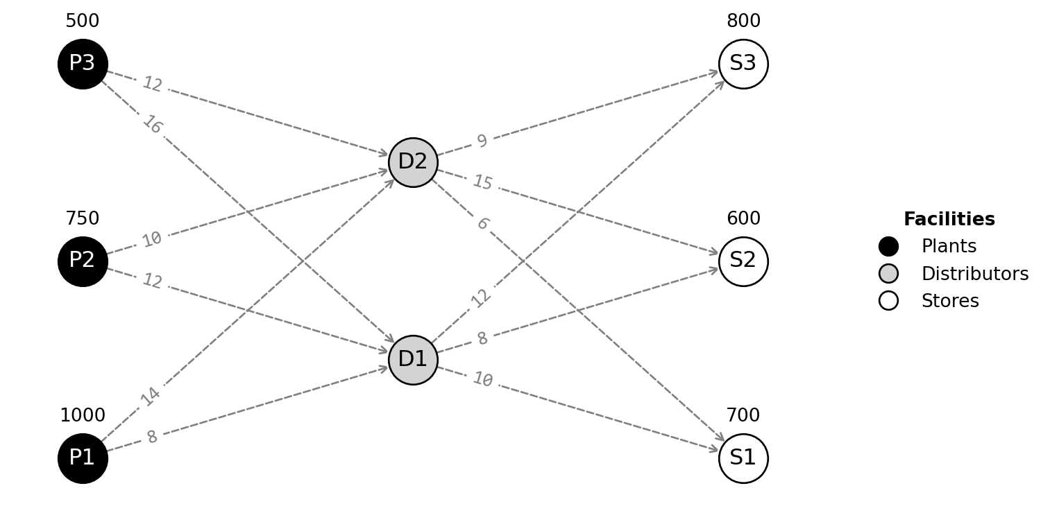
Brewery Transportation Network. Green Ale is a beer company that manages its entire transportation network. It currently operates three production plants in Enschede: one with a capacity of 1000 bottles per day (P1), another producing 750 bottles per day (P2), and a third producing 500 bottles per day (P3). The company has two distribution centers, (D1 and D2) that deliver beer to three retail stores: S1, S2, and S3. The daily demand for these stores is 700, 600, and 800 bottles, respectively. Additionally, the cost (in cents per bottle) to ship beer between locations is provided in the table below.
Question 1
Brewery Transportation Network Problem. Formulate the problem to find the optimal transportation plan for shipping beer from the breweries to the stores at minimal cost, and provide the corresponding descriptions.
Solution 1
Brewery Transportation Network Problem (Solution). The formulation is as follows:
Sets and Indices:
- \(P\): Plants
- \(D\): Distributors
- \(S\): Stores
- \(i \in P\)
- \(j \in D\)
- \(k \in S\)
Parameters:
- \(cd_{i,j}\): Cost from plant \(i\) to distributor \(j\)
- \(cs_{j,k}\): Cost from distributor \(j\) to store \(k\)
- \(d_k\): Demand at store \(k\)
- \(p_i\): Bottles produced at plant \(i\)
Variables:
- \(x_{i,j}\): Number of bottles shipped from plant \(i\) to distributor \(j\)
- \(y_{j,k}\): Number of bottles shipped from distributor \(j\) to store \(k\)
Objective: Minimize total shipping costs:
\[ \min \left( \sum_{i=1}^{3} \sum_{j=1}^{2} cd_{i,j} \cdot x_{i,j} + \sum_{j=1}^{2} \sum_{k=1}^{3} cs_{j,k} \cdot y_{j,k} \right) \]
Constraints:
- Production limit at plants: \(\sum_{j=1}^{2} x_{i,j} \leq p_i \quad \forall i\)
- Flow conservation at distributors: \(\sum_{i=1}^{3} x_{i,j} = \sum_{k=1}^{3} y_{j,k} \quad \forall j\)
- Demand satisfaction at stores: \(\sum_{j=1}^{2} y_{j,k} \geq d_k \quad \forall k\)
- Non-negativity: \(x_{i,j} \geq 0, y_{j,k} \geq 0\) for \(i \in \{1,2,3\}, j \in \{1,2\}, k \in \{1,2,3\}\)
Question 2
Brewery Transportation Network with Warehousing. Suppose the distributors want to always stockpile 250 bottles of beer to satisfy any additional and unexpected demand they may face. It costs Distributor 1 0.35 euros per bottle for daily storage and Distributor 2 0.50 euros per bottle. Formulate this case and provide the corresponding descriptions.
Solution 2
Brewery Transportation Network with Warehousing (Solution). For the scenario where distributors need to stockpile beer for unexpected demand, incorporate the following adjustments:
New Parameters Added:
- \(maxh_j\): Maximum number of bottles to be stored per day by distributor \(j\), with a maximum of 250.
- \(h_j\): Holding costs for distributor \(j\) (for \(j = 1\), it’s 0.35 euros; for \(j = 2\), it’s 0.50 euros).
New Variable Added:
- \(z_j\): Number of bottles held by distributor \(j\).
Objective Changes: Minimize the total cost including holding costs:
\[ \min \left( \sum_{i=1}^{3} \sum_{j=1}^{2} cd_{i,j} \cdot x_{i,j} + \sum_{j=1}^{2} \sum_{k=1}^{3} cs_{j,k} \cdot y_{j,k} + \sum_{j=1}^{2} z_j \cdot h_j \right) \]
Changes in Constraints:
Modify the flow conservation constraint at distributors to include storage:
\[\sum_{i=1}^{3} x_{i,j} = \sum_{k=1}^{3} y_{j,k} + z_j \quad \forall j\]
This change ensures what is received by a distributor is equal to what is dispatched to stores plus what is stored.
Add a holding constraint to the storage:
\[z_j = maxh_j \quad \forall j\]
Update the non-negativity constraint to include \(z_j\):
\[ x_{i,j} \geq 0, y_{j,k} \geq 0, z_j \geq 0 \quad \forall \, i \in \{1,2,3\}, j \in \{1,2\}, k \in \{1,2,3\} \]
Question 3
Brewery Transportation Network with Warehousing and Capacity Restrictions. The company has introduced a second type of beer to its distribution lineup. To accommodate this, they have doubled the production capacity of each plant. The three stores now have an added daily demand of 500, 600, and 700 bottles for this new product, respectively. Unfortunately, the trucks transporting the beer from the distributors to the stores can hold a maximum of 900 bottles each. Trucks travel directly from the distributor to each store (i.e., one to one). Formulate the corresponding model and provide the necessary descriptions. (1.25 points)
Solution 3
Brewery Transportation Network with Warehousing and Capacity Restrictions (Solution). The following has to be added to accommodate a new product, and maximum truck capacity and production constraints.
Sets and Indices:
- \(P\): Products
- \(m \in P\)
Parameters:
- \(cd_{i,j}\): Costs from plant \(i\) to distributor \(j\)
- \(cs_{j,k}\): Costs from distributor \(j\) to store \(k\)
- \(d_{k,m}\): Demand at store \(k\) of product \(m\)
- \(p_i\): Produced bottles at plant \(i\) (no matter what product, now doubled)
- \(maxTruck\): Max bottles that can be in a truck (= 900)
Variables:
- \(x_{i,j,m}\): amount of bottles shipped from plant \(i\) to distributor \(j\) of product \(m\)
- \(y_{j,k,m}\): amount of bottles shipped from distributor \(j\) to store \(k\) of product \(m\)
Objective:
Minimize the total cost: \[\min \left( \sum_{i = 1}^{3} \sum_{j = 1}^{2} \sum_{m=1}^{2} c_{i,j} \cdot x_{i,j,m} + \sum_{j = 1}^{2} \sum_{k = 1}^{3} \sum_{m=1}^{2} c_{j,k} \cdot y_{j,k,m} \right)\]
Constraints:
Maximum production per day:
\[\sum_{j=1}^{2} \sum_{m=1}^{2} x_{i,j,m} \leq p_i \quad \forall i\]
Conservation of flow at distributors:
\[\sum_{i=1}^{3} x_{i,j,m} = \sum_{k=1}^{3} y_{j,k,m} \quad \forall j, \forall m\]
Meeting demand per type:
\[\sum_{j=1}^{2} y_{j,k,m} \geq d_{k,m} \quad \forall k, \forall m\]
Maximum capacity in truck:
\[\sum_{m=1}^{2} y_{j,k,m} \leq maxTruck \quad \forall j, \forall k\]
Non-negativity constraints:
\[x_{i,j,m} \geq 0, y_{j,k,m} \geq 0 \quad \text{with } i \in \{1,2,3\}, j \in \{1,2\}, k \in \{1,2,3\}, m \in \{1,2\}\]
Question 4
Brewery Transportation Network and Goal Programming. You are asked to further adapt the problem formulation to incorporate the following objectives:
- Objective 1:
- the number of beers distributed from plant 1 should not exceed 450.
- the number of beers distributed from plant 2 should not exceed 450.
- Objective 2:
- the total amount of beers distributed from plant 3 should equal exactly 500.
Adjust the formulation to minimize deviations from these objectives, considering that objective (2) has higher priority than (1).
Solution 4
Brewery Transportation Network and Goal Programming (Solution). To achieve the new distribution goals:
For plants P1 and P2, minimize the deviation from the distribution cap of 450 (Objective 1):
\[\sum_{j=1}^{2} \sum_{m=1}^{2} x_{i,j,m} - d_{1i}^+ \leq 450 \quad \text{for } i \in \{1,2\}\]
For plant P3, minimize the deviation from the exact distribution requirement of 500 (Objective 2):
\[\sum_{j=1}^{2} \sum_{m=1}^{2} x_{3,j,m} + d_{2}^- - d_{2}^+ = 500\]
Additionally, ensure all variables are non-negative:
\[x_{i,j,m} \geq 0, \quad \text{for } i \in \{1,2,3\}, j \in \{1,2\}, m \in \{1,2\}\]
Given that objective (2) is of higher importance, the linear minimization (LMin) should focus on the sum of deviations for objective (2) before considering those for objective (1):
\[\text{LMin} \left( d_{2}^- + d_{2}^+, \sum d_{1i}^+ \right)\]
Scenario 2 - Truck Routing
Vehicle Routing Problem. You are tasked with addressing a truck routing problem where goods must be transported from the main depot to clients. Below is the distance matrix along with the provided information:
- There are a total of three vehicles, each with a capacity of 300, departing from the depot and returning after completing their respective routes.
- Each client can be visited only once, and upon visitation, must be fully supplied (no partial deliveries are allowed). The demand requirement for each client is 150. Every time a vehicle supplies a client, it earns a benefit of 1,000. For instance, if client 3 is visited by vehicle 1, then this vehicle will receive the corresponding 1000 in benefits for serving that client.
- All positions are reachable from any position, as illustrated by the distance matrix in Table 1.
- The cost conversion for each distance unit is 1:1. For example, moving the vehicle from the depot to client 3 costs 55.
- The time conversion for each distance unit is also 1:1 in minutes. Thus, moving from the depot to client 3 takes 55 minutes.
- The opening time of the depot is 0, and no time windows are associated with the customers.
| Depot | Client 1 | Client 2 | Client 3 | Client 4 | |
|---|---|---|---|---|---|
| From/To | |||||
| Depot | 0 | 140 | 95 | 55 | 110 |
| Client 1 | 140 | 0 | 210 | 170 | 85 |
| Client 2 | 95 | 210 | 0 | 105 | 185 |
| Client 3 | 55 | 170 | 105 | 0 | 115 |
| Client 4 | 110 | 85 | 185 | 115 | 0 |
Question 5
Vehicle Routing Problem Heuristic. You are tasked with designing and applying a constructive heuristic that prioritizes clients based on their proximity to the depot, with the goal of maximizing total profit. Describe your heuristic and demonstrate how the final solution is developed using this approach, along with the value of the objective function.
Solution 5
Vehicle Routing Problem Heuristic (Solution). To solve this question you are required to provide either a pseudocode or a flowchart, followed by a demonstration of how a solution is constructed using your proposed method. It’s crucial that your pseudocode is detailed enough to enable the construction of the solution without omitting any steps. The clarity and completeness of your pseudocode should allow for the replication of the same solution you achieved.
Question 6
Vehicle Routing Problem Reoptimization. Consider the solution obtained from the previous exercise, with the assumption that time starts at \(t=0\). Suppose that at time \(t=35\), you receive information indicating that all motorways to and from Client 1 are congested, resulting in an increase of 20 units for all distances related to that client. For example, the distance from Client 1 to Client 4 now becomes 105 units. Additionally, at time \(t=60\), a new client (Client 5), requiring the same demand as the other clients, emerges and must be served. The distance to all clients and the depot from Client 5 is 50 units.
If service is not provided, a penalty of 200 is incurred. Design and describe an instant reoptimization approach using the nearest neighbor heuristic, and calculate the resilience for each case (i.e., \(t=35\) and \(t=60\)). Consider that if a vehicle is en route to a client, this client can no longer be disrupted; reoptimization is only possible after visiting this client.
What is the benefit of reoptimizing in each case? Provide the necessary calculations and explanations.
Solution 6
Vehicle Routing Problem Reoptimization (Solution). This analysis depends on your previously obtained solution.
Initial Solution:
Let’s assume we obtain the following solution (Distance=590, Revenue=4,000, Profit=3,410):
Vehicle 1:
[Depot]----55---->[Client 3]---105---->[Client 2]----95---->[Depot](Distance=255, Revenue=2,000, Profit=1,745)Vehicle 2:
[Depot]---110---->[Client 4]----85---->[Client 1]---140---->[Depot](Distance=335, Revenue=2,000, Profit=1,665)Vehicle 3:
[Depot]----0----->[Depot](Distance=0, Revenue=0, Profit=0)
Disruption 1 (\(t=35\)):
At \(t=35\), Vehicle 1 is en route to Client 3 and, subsequently, will proceed to Client 2. Conversely, Vehicle 2 is on its way to Client 4 and then to Client 1.
Every change in the route will result in the same outcome since all paths to/from Client 1 receive an increase of 20. Moreover, when we become aware of this event, Vehicle 2 is still en route to Client 4. It is important to note that we are applying the optimization of the same heuristic, nearest neighbor. Client 1 remains the closest to Client 4 due to the uniform increase in paths to it.
| Depot | Client 1 | Client 2 | Client 3 | Client 4 | Client 5 | |
|---|---|---|---|---|---|---|
| From/To | ||||||
| Depot | 0 | 160 | 95 | 55 | 110 | 50 |
| Client 1 | 160 | 0 | 230 | 190 | 105 | 50 |
| Client 2 | 95 | 230 | 0 | 105 | 185 | 50 |
| Client 3 | 55 | 190 | 105 | 0 | 115 | 50 |
| Client 4 | 110 | 105 | 185 | 115 | 0 | 50 |
| Client 5 | 50 | 50 | 50 | 50 | 50 | 0 |
Disrupted Solution = Recovered Solution (Distance=630, Revenue=4,000, Profit=3,370):
Vehicle 1:
[Depot]----55---->[Client 3]---105---->[Client 2]----95---->[Depot](Distance=255, Revenue=2,000, Profit=1,745)Vehicle 2:
[Depot]---110---->[Client 4]---105---->[Client 1]---160---->[Depot](Distance=375, Revenue=2,000, Profit=1,625)Vehicle 3:
[Depot]----0----->[Depot](Distance=0, Revenue=0, Profit=0)
Therefore, Vehicle 2 route is increased by 40: 20 for leg (4,1) and 20 for leg (1,Depot).
Resilience Formula
\[ \text{Resilience} = \frac{(\text{Disrupted Solution} - \text{Recovered Solution})}{(\text{Disrupted Solution} - \text{Initial Solution})} \]
See details on resilience calculation in (Pant et al. 2014).
\[\text{Resilience} = \frac{(3370 - 3370)}{(3370 - 3410)} = -0.00\]
As you can see, the value is 0; we cannot do anything (with the current options) to recover to the previous state. This indicates that this type of event is beyond our management. However, after observing this event, we can take it into account for future operations and include additional recovery options to also cover this type of event.
Disruption 2 (\(t=60\)):
At \(t=60\), a new client arrives with the same demand and a distance of 50 to each client and depot. The initial cost is 3,370, the same as the solution after the event described above. If doing nothing, the cost becomes 3,170 (due to the 200 rejection penalty). During reoptimization at \(t=60\), we find ourselves in the following situation:
- Vehicle 1 is carrying Client 3 (load = 150) and on its way to Client 2, arriving at \(t=55+105\).
- Vehicle 2 is empty and on its way to Client 4, arriving at \(t=110\).
- Vehicle 3 is empty and idle at the depot.
Given the circumstances:
- Vehicle 1 cannot pick up other clients since it is already en route to Client 2. Upon picking up this client, maximum capacity (300) will be reached.
- Vehicle 2 route can be re-optimized when it arrives at Client 4 at \(t=110\).
- Vehicle 3 can be assigned to clients.
Following the nearest neighbor approach, and depending on the order vehicles are selected for reoptimization we have two possible options:
Option 1. Re-optimize Vehicle 2 (Distance=730, Revenue=5,000, Profit=4,270):
Vehicle 1:
[Depot]----55---->[Client 3]---105---->[Client 2]----95---->[Depot](Distance=255, Revenue=2,000, Profit=1,745)Vehicle 2:
[Depot]---110---->[Client 4]---105---->[Client 1]---160---->[Depot](Distance=375, Revenue=2,000, Profit=1,625)Vehicle 3:
[Depot]----50---->[Client 5]----50---->[Depot](Distance=100, Revenue=1,000, Profit=900)
\[\text{Resilience} = \frac{(3170 - 4270)}{(3170 - 3370)} = 5.50\]
Option 2. Do not re-optimize Vehicle 2 (Distance=785, Revenue=5,000, Profit=4,215):
Vehicle 1:
[Depot]----55---->[Client 3]---105---->[Client 2]----95---->[Depot](Distance=255, Revenue=2,000, Profit=1,745)Vehicle 2:
[Depot]---110---->[Client 4]----50---->[Client 5]----50---->[Depot](Distance=210, Revenue=2,000, Profit=1,790)Vehicle 3:
[Depot]---160---->[Client 1]---160---->[Depot](Distance=320, Revenue=1,000, Profit=680)
\[\text{Resilience} = \frac{(3170 - 4215)}{(3170 - 3370)} = 5.22\]
A resilience factor equal to 1 indicates full recovery. However, here we observe factors greater than 1, indicating that we have improved the initial state. This improvement occurs when our actions not only recover from the previous state but also enhance the situation by leveraging the event that occurred.
Question 7
Collaborative Logistics. You now face a scenario where each vehicle is associated with a specific client. For example, Vehicle 1, operating independently, can only serve Client 1.
Approach this situation as a cooperative game and calculate the Shapley allocation for this particular case. Use the nearest neighbor heuristic to determine the profit values of the coalitions (e.g., \(v(\{1\})\), \(v(\{1,2\})\), etc.). When the coalition includes more than one vehicle, the vehicle closest to the next client will be selected for service. For instance, in a coalition of two vehicles, after the first vehicle visits the nearest client to the depot, the subsequent client will be served by the vehicle that is closest to that client from its current position. Provide the necessary calculations and explanations. Lastly, verify whether the solution resides within the core; if it does not, suggest an extension to include the solution.
| Client | Associated vehicle | |
|---|---|---|
| 0 | 1 | 1 |
| 1 | 2 | 2 |
| 2 | 3 | 2 |
| 3 | 4 | 3 |
Shapley Value Formula
\[Sh_i = \sum_{S \subseteq N \setminus \{i\}} \frac{|S|! \big(n - |S| - 1\big)!}{n!} \cdot \big(v(S \cup \{i\}) - v(S)\big)\]
Core Formula
\[C(N,v) = \left\{ p \in \mathbb{R}^N \middle| \sum_{i \in N} p^i = v(N),\ \forall S \subseteq N, S \neq \emptyset : \sum_{i \in S} p^i \geq v(S) \right\}\]
Solution 7
Collaborative Logistics (Solution). Solution procedure:
- Use your routing algorithm to calculate \(v({1})\), \(v({2})\), \(v({3})\), \(v({1,3})\), \(v({2,3})\), and \(v({1,2,3})\).
- Obtain the Shapley values:
- Calculate \(q\) values \(q_1, q_2, q_3\) for each vehicle.
- Calculate marginal contributions \(\phi_1\), \(\phi_2\), \(\phi_3\) for each vehicle.
- Once you have all Shapley values, compare them to ensure they are not worse than the individual \(V\) values, that is, check if the solution is in the core (efficiency and stability).
- If the solution is not in the core, the instability can be overcome by making sure an allocation is in the \(\epsilon\)-core, so it is not possible for any coalition to provide its members with a benefit exceeding what they already receive from the allocation by more than \(\epsilon\).
Background
Shapley Value Formula
The general formula for the Shapley value for a player \(i\) in a game with \(n\) players:
\[Sh_i = \sum_{S \subseteq N \setminus \{i\}} \frac{|S|! (n - |S| - 1)!}{n!} \cdot (v(S \cup \{i\}) - v(S))\]
Where:
- \(Sh_i\) is the Shapley value for player \(i\).
- \(N\) is the set of all players.
- \(S\) is a subset of players without player \(i\).
- \(|S|\) is the number of players in subset \(S\).
- \(n\) is the total number of players.
- \(v(S)\) is the value of the coalition \(S\).
- The factorial terms \(|S|! (n - |S| - 1)!\) and \(n!\) represent the number of permutations of players joining before and after player \(i\), and the total number of permutations, respectively.
The term \(v(S \cup \{i\}) - v(S)\) in the Shapley value formula represents the marginal contribution of player \(i\) to the coalition \(S\).
- \(v(S)\) is the value (or payoff) of the coalition \(S\) before player \(i\) joins. It reflects the total benefit that the members of \(S\) can achieve by cooperating without the involvement of player \(i\).
- \(v(S \cup \{i\})\) is the value of the coalition formed by adding player \(i\) to the existing coalition \(S\), indicating the total benefit that the members of \(S\), along with player \(i\), can achieve by cooperating.
- The difference \(v(S \cup \{i\}) - v(S)\) calculates the incremental value or benefit that player \(i\) brings to the coalition \(S\). It quantifies how much more the coalition \(S\) is worth with player \(i\) than without them.
The fraction
\[ q(|S|) = \frac{|S|! \cdot (n - |S| - 1)!}{n!} \]
is called the Shapley weight. It accounts for the number of permutations where coalition \(S\) appears just before player \(i\) in the order of joining. This reflects how likely player \(i\) is to join a group of size \(|S|\) if everyone joins in a random order.
Shapley Value Properties
The Shapley allocation ensures that the following properties are satisfied:
Efficiency. The complete utility is distributed among all the players. This means that there is no excess or shortfall in allocation.
Symmetry. If two players provide the same contribution to a coalition not containing both of them, then their corresponding value is the same. This ensures that the allocation is not influenced by external factors such as negotiation power or historical precedence, maintaining fairness and impartiality in distribution.
Dummy Player. A dummy-player, a player that contributes nothing to any coalition, receives what the player can achieve by himself. This ensures that non-contributors are not unfairly rewarded.
Formally:
Efficiency. The sum of all players’ payoffs \(p^i\) must equal the total value of the grand coalition \(v(N)\):
\[ \sum_{i \in N} p^i = v(N). \]
Symmetry. If two players \(i\) and \(j\) contribute equally to any coalition \(S\) (i.e., \(i\) and \(j\) are interchangeable), their allocated values should also be equal.
\[ v(S \cup \{i\}) = v(S \cup \{j\}) \quad \forall S, \, \text{such that} \ i,j \notin S \]
Dummy Player. For a dummy player \(i\), their contribution to any coalition \(S\) equals their own value acting alone, \(v(\{i\})\):
\[ v(S \cup \{i\}) - v(S) = v(\{i\}) \quad \forall S, \, \text{such that} \ i \notin S \]
Core Formula
The core of a the game is represented as: \[C(N,v) = \left\{ p \in \mathbb{R}^N \middle| \sum_{i \in N} p^i = v(N),\ \forall S \subseteq N, S \neq \emptyset : \sum_{i \in S} p^i \geq v(S) \right\}\]
Where:
- \(C(N,v)\): Set of payoff distributions among players.
- \(N\): Set of all players in the game.
- \(v\): A function that assigns a value to every coalition \(S\). The value \(v(S)\) is the total worth that coalition \(S\) can achieve by itself.
- \(p\): A vector of proposed payoffs \(p^i\) for each player \(i\).
- \(\mathbb{R}^N\): The N-dimensional real space, which in this context represents all possible distributions of payoffs among the N players.
The conditions defined within the curly braces are as follows:
- \(\sum_{i \in N} p^i = v(N)\): The total payoffs distributed among all players must equal the total worth of the grand coalition (the coalition of all players). (Efficiency Condition).
- \(\sum_{i \in S} p^i \geq v(S)\): The sum of payoffs to the members of coalition \(S\) must be at least as large as the value that coalition can achieve on its own. This way, no subset of players has an incentive to break away from the grand coalition since they cannot do better by themselves (Stability Condition).
Core Properties
Efficiency. The sum of individual payoffs \(p^i\) for all players \(i\) in the grand coalition \(N\) is equal to the total value \(v(N)\) of the coalition.
\[ \sum_{i \in N} p^i = v(N) \]
Coalitional Rationality / Stability. For every subset \(S\) of the grand coalition \(N\), the sum of the payoffs to the members of \(S\) is at least as large as the value that \(S\) could achieve on its own.
\[ \sum_{i \in S} p^i \geq v(S), \forall S \subseteq N \]
Having a cost/profit allocation in the core ensures that the following properties are satisfied:
- Efficiency. All the value created by the coalition is distributed among its members without any surplus or deficit.
- Coalitional Rationality / Stability. No subgroup of players has an incentive to break away from the grand coalition, as they cannot achieve a better outcome by doing so.
In the following, we will implement steps 1-3.
These steps are implemented below (Click on the blocks to see calculation details).
Coalition’s Profits. Expected payoffs \(v(S)\) of coalitions \(S\) of players \(N = \{1, 2, 3\}\)
Shapley’s Profit Allocation. \(\phi = (782.50, 1727.50, 855.00)\)
Shapley Value Formula
\[\phi_i = \sum_{S \subseteq N \setminus \{i\}} \frac{|S|! \big(n - |S| - 1\big)!}{n!} \cdot \big[v(S \cup \{i\}) - v(S)\big]\]
Core Check. Allocation (782.50, 1727.50, 855.00) is not in the core (\(\epsilon = 27.5\))
References
Pant, Rajat, Kash Barker, Jos’e Emmanuel Ram’irez-Marquez, and Claudio M Rocco. 2014. “Stochastic Measures of Resilience and Their Application to Container Terminals.” Computers & Industrial Engineering 70: 183–94. https://doi.org/10.1016/j.cie.2014.01.017.